Efficient Unified Stokes using a Polynomial Reduced Fluid Model
Abstract
Unsteady Stokes solvers, coupling stress and pressure forces, are a key component of accurate free surface simulators for highly viscous fluids. Because of the simultaneous application of stress and pressure terms, this creates a much larger system than the standard decoupled approach. We propose a reduced fluid model wherein interior regions are represented with incompressible polynomial vector fields. Sets of standard grid cells are consolidated into super-cells, each of which are modelled using only 26 degrees of freedom. This reduced model retains desirable behaviour of the full Stokes system with smaller computational cost.
Presentation
Full Text
Full text is published at https://diglib.eg.org/handle/10.2312/sca20201214.
Introduction
Accurate coupling of pressure and viscous shear stresses are necessary for simulation of strongly viscous liquids, as highlighted by the liquid rope coiling instability. Standard decoupled methods have trouble simulating such phenomena, while unified Stokes solvers are effective but create much larger systems leading to higher computational costs [LBB2017]. Spatial adaptivity can be used to reduce computational cost by concentrating workload on the fluid surface where most visual effects are found. [GAB20] proposed a spatial coarsening method for pressure projection whereby a set of interior cells are consolidated into a coarsened super-cell, whose velocity is defined using an incompressible affine vector field.
Building on these ideas, we propose a unified Stokes solver featuring interior regions described using an incompressible polynomial vector field, primarily of degree 2. We show that an affine model is insufficient for the Stokes problem, and that the quadratic model is required for proper resolution of viscous forces while being small enough to provide increased computational efficiency.
Fluid Equations
We seek to solve the following system for unsteady Stokes flow:
\[\begin{align} \frac{\mathbf{u}_{n+1}-\mathbf{u}^*}{\Delta{}t} &= \frac{1}{\rho{}}\left( -\nabla{}p + \nabla\cdot\mathbf{\tau} \right) \label{eq:1} \\ \nabla\cdot\mathbf{u}_{n+1} &= 0 \\ \mathbf{\tau} &= \mu\left( \nabla\mathbf{u}_{n+1} + (\nabla{}\mathbf{u}_{n+1})^T \right) \end{align}\]where \(\mathbf{u}\) is the velocity field, \(\mathbf{\tau}\) is the symmetric deviatoric stress tensor, \(\mu\) is the dynamic viscosity coefficient, \(\rho\) is density, \(p\) is pressure, \(\Delta{}t\) is the timestep size, and subscripts represent evaluation of a variable at that timestep.
Discretizing using the variational form following [LBB2017] gives:
\[\begin{align} \begin{bmatrix} \frac{1}{\Delta{}t}\mathbf{M} W_F^uW_L^u & W_F^u\mathbf{G}W_L^p & W_F^u\mathbf{D}^TW_L^\tau{} \\ W_L^p\mathbf{G}^TW_F^u & 0 & 0 \\ W_L^\tau{}\mathbf{D}W_{F}^u & 0 & -\frac{1}{2}\mathbf{\mu}^{-1}W_F^\tau{}W_L^\tau{} \end{bmatrix} \begin{bmatrix} \mathbf{u} \\ \mathbf{p} \\ \mathbf{\tau} \end{bmatrix} &= \begin{bmatrix} \frac{1}{\Delta{}t}\mathbf{M} W_F^uW_L^u\mathbf{u}^* \\ 0 \\ 0 \end{bmatrix} \label{eq:discreteStokes} \end{align}\]where \(\mathbf{u}\), \(\mathbf{\tau}\), and \(\mathbf{p}\) are stacked velocities, stresses, and pressure components respectively, \(\mathbf{M}\) is the diagonal matrix of densities per velocity sample, \(\mathbf{\mu}\) is the diagonal matrix of viscosity coefficients per stress sample, \(\mathbf{G}\) is the discrete gradient operator, \(\mathbf{D}\) is discrete deformation rate operator with \(\mathbf{D}\mathbf{u}=\frac{1}{2}\left(\nabla{}\mathbf{u}+(\nabla{}\mathbf{u})^T\right)\).
Polynomial Velocity Field
For a fluid region \(\Omega_B\), we define the following quadratic field,
\[\begin{align} \mathbf{u}_{B}(\mathbf{x}) = \mathbf{u}_{const} + \mathcal{G}(\mathbf{x}-\mathbf{x}_{COM}) + \frac{1}{2}(\mathbf{x}-\mathbf{x}_{COM})^T\mathcal{H}(\mathbf{x}-\mathbf{x}_{COM}) \end{align}\]where \(\mathbf{x}_{COM}\) is the center of mass (or any stationary reference point) of \(\Omega_B\), \(\mathcal{G} = \nabla\mathbf{u}_B\) is the gradient 2-tensor, and \(\mathcal{H} = \nabla(\nabla\mathbf{u}_B)\) is the Hessian 3-tensor with \(\mathcal{H}_{i,j,k} = \frac{\partial^2u_i}{\partial{}x_j\partial{}x_k}\). Each page \(i\) of \(\mathcal{H}\) is symmetric, thus requiring only 18 degrees of freedom rather than the full 27. We enforce incompressibility by applying the usual \(\nabla\cdot\mathbf{u}_B=0\) constraint, further reducing the degrees of freedom to 26: 3 for the constant term, 8 for the linear term, and 15 for the quadratic term.
Thus, the velocity within each region \(\Omega_B\) can be described by a generalized velocity vector \(\mathbf{v}_B\) of 26 elements. We define a matrix \(\mathbf{C}\) that gives the Euclidean velocity at any point \(\mathbf{x}\). For brevity, we elucidate the 2D case with the 3D case following straightforwardly:
\[\begin{align} \mathbf{u}_{B} &= \mathbf{C}(\mathbf{x})\mathbf{v}_B \\ &= \begin{bmatrix} 1 & 0 & \tilde{x} & \tilde{y} & 0 & \tilde{x}^2 & \tilde{y}^2 & 0 & -2\tilde{x}\tilde{y} \\ 0 & 1 & -\tilde{y} & 0 & \tilde{x} & -2\tilde{x}\tilde{y} & 0 & \tilde{x}^2 & \tilde{y}^2 \end{bmatrix}\mathbf{v}_{B} \label{eq:C} \end{align}\]where \(\tilde{x} = x-x_{COM}\) and similarly for \(\tilde{y}\). Henceforth, we use this quadratic model; changing the definition of \(\mathbf{C}\) allows for flexible generalization to higher order with freedom to choose which modes to include. Using this transformation, a generalized mass matrix can be defined as follows:
\[\begin{align} \mathbf{M}_{B} = \iiint_{\Omega_B} \rho_B\mathbf{C}^T\mathbf{C} dV \label{eq:generalizedMass} \end{align}\]Coupling to Regular Grid
We wish to couple this quadratic field to a regular grid, applying the reduced model in the interior and the regular grid solver to the boundary regions of the fluid. To do so, we define a transfer matrix \(\mathbf{J}:\mathbf{u}_B\rightarrow{}\mathbf{v}_B\) which accumulates forces from the regular grid and transforms them into generalized forces applicable to the interior regions:
\[\begin{align} \mathbf{J}\mathbf{f} = \sum_{a,j}\mathbf{C}_a(\mathbf{x}_j)^T \mathbf{f}_j \end{align}\]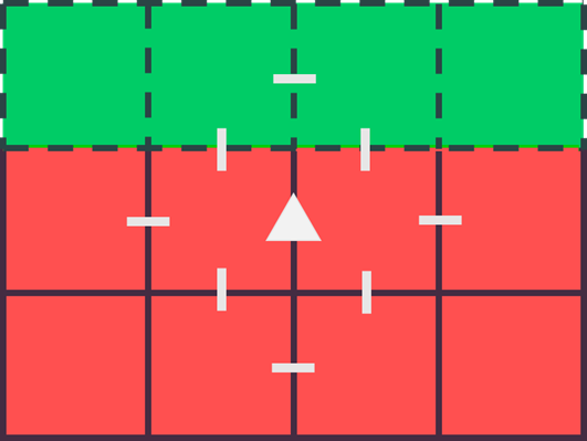
Inset 1:
where \(a\) iterates over each axis, \(j\) iterates over boundary faces, \(\mathbf{x}_j\) is the center of face \(j\), and \(\mathbf{f}_j\) is a force in Cartesian form. As shown by the inset figure, the stress stencil (white dashes) of a velocity sample (triangle) may include perpendicular faces touching the boundary, which must also be counted in \(j\). Regular grid cells are in red, interior cells in green, and dashed lines indicate velocities defined by the reduced model. The \(\mathbf{J}^T\) transpose operation distributes generalized forces into the surrounding regular grid representation.
Applying our reduced model and the transformation between the two representations to Equation \ref{eq:discreteStokes}, we arrive at:
\[\begin{align} \nonumber \begin{bmatrix} \frac{1}{\Delta{}t}\mathbf{M}_F W_F^uW_L^u & 0 & W_F^u\mathbf{G}W_L^p & W_F^u\mathbf{D}^TW_L^\tau{} \\ 0 & \frac{1}{\Delta{}t}\mathbf{M}_B + \mathbf{J}\mathbf{D}^T\mathbf{D}\mathbf{J}^T & \mathbf{J}W_F^u\mathbf{G}W_L^p & \mathbf{J}W_F^u\mathbf{D}^TW_L^\tau{} \\ W_L^p\mathbf{G}^TW_F^u & W_L^p\mathbf{G}^TW_F^u\mathbf{J}^T & 0 & 0 \\ W_L^\tau{}\mathbf{D}W_{F}^u & W_L^\tau{}\mathbf{D}W_{F}^u\mathbf{J}^T & 0 & -\frac{1}{2}\mathbf{\mu}^{-1}W_F^\tau{}W_L^\tau{} \end{bmatrix} \begin{bmatrix} \mathbf{u}_F \\ \mathbf{v}_B \\ \mathbf{p} \\ \mathbf{\tau} \end{bmatrix} \\ = \begin{bmatrix} \frac{1}{\Delta{}t}\mathbf{M}_F W_F^uW_L^u\mathbf{u}_F^* \\ \frac{1}{\Delta{}t}\mathbf{M}_B\mathbf{v}_B^* \\ 0 \\ 0 \end{bmatrix} \label{eq:fullsystem} \end{align}\]where \(\mathbf{M}_F\) is the diagonal matrix of densities, \(\mathbf{u}_F\) are Cartesian velocities being solved for, and \(\mathbf{u}_F^*\) is the input Cartesian velocities, all defined solely for regular grid cells. Analogously, \(\mathbf{M}_B\) is the generalized mass matrix defined in Equation \ref{eq:generalizedMass}, \(\mathbf{v}_B\) are generalized velocities being solved for, and \(\mathbf{v}_B^*\) are input generalized velocities, all defined solely for interior regions. This matrix is amenable to transformation into more convenient forms via Schur complements. For our results, we eliminated stress to produce a pressure-velocity form that allows for easiest implementation, avoiding construction of the dual grid for stresses. Alternatively, eliminating velocities produces a symmetric positive-definite system, but requires the inversion of each interior region block (a \(26\times{}26\) matrix).
Notice that, in effect, we are solving for Equation \ref{eq:1} separately for the regular grid cells and interior regions, with coupling being handled by the stress and pressure forces being applied on the boundary. Incompressibility of interior regions is handled implicitly by the definition of our reduced model. In practice, we simply perform the usual iteration through all faces using the usual stencils for \(\mathbf{G}\) and \(\mathbf{D}\), with faces that fall inside the interior regions being replaced by generalized variables transformed using \(\mathbf{J}^T\). This allows for very straightforward implementation into existing grid solvers.
Tiled Interior Regions
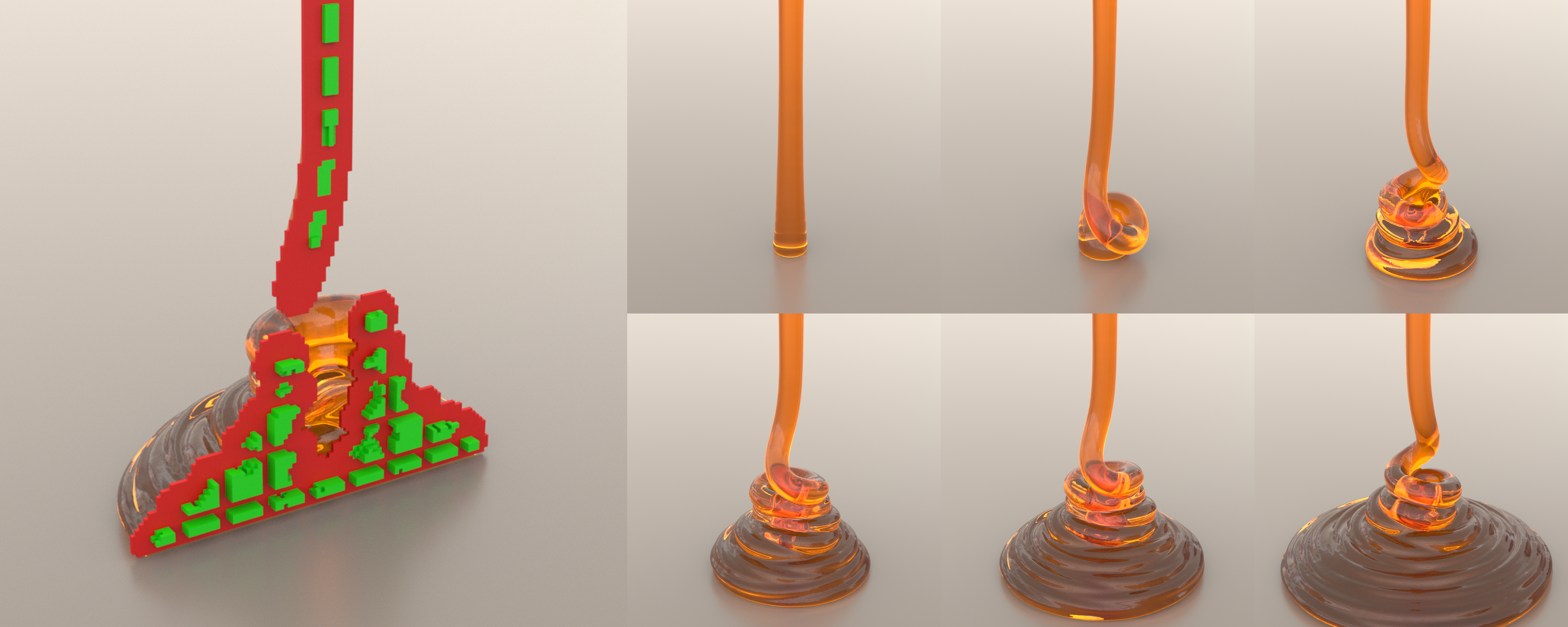
Figure 1: Liquid rope coiling instability solved using tiled quadratic regions of size \(7^3\), with 3-cell padding between. Cutaway view shown on the left, featuring regular grid cells in red and our reduced model interior regions in green.
Although the defined quadratic regions are highly expressive, they nonetheless have a limited space of representable fields. As such, following [GAB20], we apply a tiling approach where we limit the size of interior regions to a user-defined constant, with a layer of regular grid cells between, shown on Figure 1. Due to the size of the viscous operator (\(\mathbf{D}^T\mathbf{D}\)), we recommend that the padding between interior regions be at least two regular grid cells wide, to prevent the stencils of one region to reach into another. This is not a strict rule–a padding size of 1 is possible but it mutually couples neighbouring interior regions together, ruling out the use of the SPD form as well as hampering performance in the non-SPD form. We also observe that interacting interior regions result in much less lively results with greater apparent viscosity, as interior regions become limited in their dynamics by the viscous stencils of neighbouring regions.
Results and Discussion
Liquid Rope Coiling
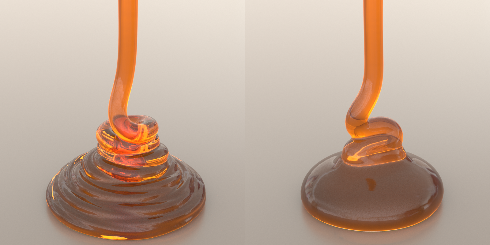
Figure 2: Comparison between the unified Stokes (left) and the decoupled approaches (right), both using our reduced fluid model.
We demonstrate that we retain the desirable free surface accuracy of a fully uniform Stokes approach by replicating the liquid rope coiling instability, shown on Figure 1. Proper resolution of the instability requires simultaneous solution of pressure and viscous forces, shown on Figure 2. This figure also demonstrates our reduced model works for decoupled methods, where we remove the pressure terms from Equation \ref{eq:fullsystem} to construct just the viscosity step [TL19]. Here, we get expected behaviour for decoupled methods, producing a falling stream that randomly buckles rather than the desired cylindrical coil, in addition to reduced surface detail [BB08].
Viscous Beam
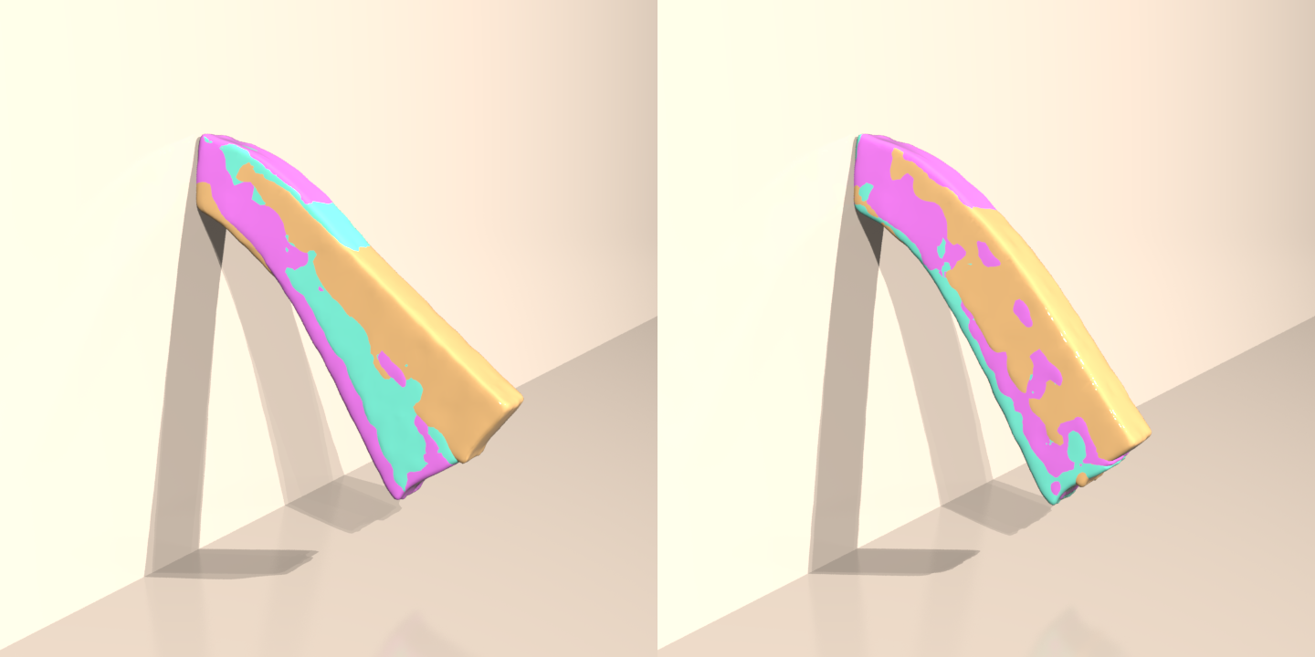
Figure 3: Overlaid viscous beams using (pink) uniform grid, (blue) quadratic regions, and (orange) affine regions. Left image uses one interior region and right image features tiled regions of size \(16^3\).
We highlight the effectiveness of the quadratic model over a potential affine model (consisting of the first \(5\) columns of \(\mathbf{C}\) from Equation \ref{eq:C}) with a viscous beam collapsing under gravity (\(\rho{}=1\), \(\mu{}=10\)), shown on Figure 3. The quadratic model accurately captures the same solution as a fully uniform solver, while affine regions result in spurious stiffness. We emphasize that this is not because the affine model cannot represent the velocity fields for this problem; the fields are simple enough that a visually satisfactory fit does exist. Rather, an affine representation does not have enough information to evolve itself–the affine assumption means that the second derivative of velocity is always zero, completely removing the viscous stress term. Applying tiling partially alleviates the issue, but the affine method still does not converge to the same solution as a fully uniform solver. Once again, this suggests the issue lies not with the reduced model reconstruction, as keeping a constant tile size means each tile represents a physically smaller space (and consequently a more affine-like field) as resolution increases.
Error and Convergence
We demonstrate error and convergence using a 2D analytical test case consisting of a fluid disk of radius \(r=0.75\), \(\rho{}=1\), \(\mu=0.1\) evolved over \(\Delta{}t=1\). We define a final velocity field as \(u = \nabla\times\frac{128}{81}r^4\cos(2\theta)\cos(\sqrt{3}\ln{}r)(15-30r+16r^2)\). The initial condition can be found by analytically evolving the final velocity backwards. As expected, results (Table 1) demonstrate that error using our reduced model is considerably larger than with a uniform grid, as well as verifying approximately second order convergence. We highlight, however, the dramatic difference in computation time, especially at higher resolutions. Comparing the reduced model’s \(128^2\) solution to the uniform grid’s \(64^2\), we see that the resulting errors are similar, yet our reduced model yields a higher resolution for similar computation time. Considering that error scales at high resolutions are imperceptibly small, we conclude that our method makes physically plausible high resolution simulation of Stokes flow much more practical than previously possible.
Table 1: Error and timing comparison for a fluid disk with known analytical solution.
| Uniform Grid | Tiled Interior Size \(16^3\) | |||||
|---|---|---|---|---|---|---|
| dx | \(L_1\) | \(L_\infty\) | Time(s) | \(L_1\) | \(L_\infty\) | Time(s) |
| \(1/32\) | 0.0226 | 0.0319 | 7.4 | 1.151 | 0.727 | 3.8 |
| \(1/64\) | 0.0110 | 0.0230 | 101 | 0.1150 | 0.1248 | 22 |
| \(1/128\) | 0.00588 | 0.0144 | 2740 | 0.0205 | 0.0256 | 111 |
References
[BB08] BATTY C., BRIDSON R.: Accurate viscous free surfaces for buckling, coiling, and rotating liquids. In Symposium on Computer Animation (2008), pp. 219–228. 3
[GAB20] GOLDADE R., AANJANEYA M., BATTY C.: Constraint bubbles and affine regions: Reduced fluid models for efficient immersed bubbles and flexible spatial coarsening. ACM Transactions on Graphics (TOG) 39, 4 (2020), 43–1. 1, 2
[LBB17] LARIONOV E., BATTY C., BRIDSON R.: Variational stokes: A unified pressure-viscosity solver for accurate viscous liquids. ACMTransactions on Graphics (TOG) 36, 4 (2017), 1–11. 1, 2
[TL19] TAKAHASHI T., LIN M. C.: A geometrically consistent viscous fluid solver with two-way fluid-solid coupling. In Computer Graphics Forum (2019), vol. 38, Wiley Online Library, pp. 49–58. 3