Low shear diffusion central schemes for particle methods
Abstract
We present the first application of a central scheme in an unstructured meshless code and extend it to limit diffusion in shearing flows.
Some numerical diffusion is required in simulations of compressible fluids to maintain stability and prevent formation of spurious structures. The Kurganov-Tadmor (KT) central scheme uses a signal velocity and a linear reconstruction of fields to limit numerical diffusion away from discontinuities.
We implement the KT scheme as a drop-in replacement for the Riemann solver in the GIZMO hydrodynamics code. Both the original finite-volume version of the KT scheme, which is quasi-Lagrangian in meshless geometry, as well as a new fully-Lagrangian finite-mass variant are presented. In addition, to mitigate excessive diffusion, a new shear-based switch is proposed. The new methods, as well as the default Riemann solver, were applied to a set of test problems. The results show that, although the KT scheme is more diffusive than the Riemann solver, it produces correct results with better convergence. The switch is shown to reduce diffusion in shearing cases, while not compromising stability in the supersonic regime. The fully-Lagrangian variant is shown to behave similarly to its Riemann solver counterpart. We conclude that the new variants of the KT scheme are good alternatives to Riemann solvers in meshless geometry, especially where its simplicity is desirable, such as for a complex equation of state.
Full Text
Full text is published on https://doi.org/10.1016/j.jcp.2020.109454.
Introducton
In this paper, we aim to solve the following hyperbolic conservation law,
\[\begin{align} \frac{\partial}{\partial{}t}\mathbf{U}(\mathbf{x},t) + \nabla\cdot\mathbf{F}(\mathbf{x},t) &= 0 \label{eq:generalform} \end{align}\]where \(\mathbf{U}\) is the vector of conserved quantities, and \(\mathbf{F}\) is the nonlinear convective flux. Of particular interest is the application to inviscid, incompressible gases, for which \(\mathbf{U}\) is the fluid state,
\[\begin{align} \mathbf{U} &= \begin{bmatrix}\rho & \rho{}v_x & \rho{}v_y & \rho{}v_z & \rho{}e_T\end{bmatrix}^T \end{align}\]and \(\mathbf{F}\) defines the fluxes across a plane with unit normal vector \(\mathbf{n} = [n_x \ n_y \ n_z]^T\):
\[\begin{align} \mathbf{F} &= \begin{bmatrix} \rho{}v_n \\ \rho{}v_x{}v_n + Pn_x \\ \rho{}v_y{}v_n + Pn_y \\ \rho{}v_z{}v_n + Pn_z \\ \rho{}v_n(e_T + \frac{P}{\rho}) \end{bmatrix} \end{align}\]Here, \(\rho\) is density, \(P\) is pressure, \(\mathbf{v}=[v_x\ v_y\ v_z]^T\) is the velocity vector, \(v_n = \mathbf{v}\cdot{}\mathbf{n}\) is its scalar projection onto \(\mathbf{n}\), and \(e_T = e + \frac{1}{2}\|\mathbf{v}\|^2\) is the specific total energy. An equation of state such as \(P=(\gamma{}-1)\rho{}e\) for ideal gases completes the system. We note, however, that our method is independent of the choice of equation of state.
In the following work, we propose a method for solving the above problem in an unstructured meshless geometry. In particular, we demonstrate the viability of the Kurganov-Tadmor (KT) central scheme [1] to compute finite-volume Godunov-like fluxes in said geometry. This, in effect, acts as a replacement for Riemann solvers, simplifying implementation and suggesting applicability to any general finite-volume geometry. We additionally derive a novel finite-mass extension of the KT scheme, as well as propose a new numerical diffusion switch based on splitting the numerical flux between a shearing and a normal component.
Background
Meshless Discretization
We assume a meshless geometry defined by a set of particles, as prescribed in the work of Gaburov & Nitadori [2], which aims to combine desirable properties from both grid and particle methods. This method builds on progress from Onate et. al. [4] which introduced the moving least-squares interpolation to computational mechanics, Dilts 1999 [5] which produced a smoothed particle hydrodynamics (SPH) implementation, and Lanson & Vila [6] which introduced meshless particle area and gradient estimators. To this, Gaburov & Nitadori introduced a Riemann solver to compute fluxes between pairwise interacting particles, completing a Godunov-style finite-volume framework.
Broadly, this meshless method provides a kernel-based reconstruction similar to SPH. A key distinction of the meshless method is that it reconstructs a face area and normal, which allows it to discretize the hyperbolic conservation law (Equation \ref{eq:generalform}) as a Godunov-like form [6, 2]. This means pairwise fluxes between particles can be computed using a numerical flux function and the approximate face area. Implementations often compute numerical fluxes via a slope reconstruction to project the fluid state to the faces then use a Riemann solver at the face [2,3] – we later show this can be replaced with a central scheme formulation.
We briefly review the derivation of this meshless discretization, following closely Section 2.1 of [2], but also refer the reader to Section 2.2 of [6] and Section 2.1 of [3] for a more complete discussion. Following the usual finite-volume derivation, we seek a solution of the weak form of the hyperbolic conservation law Equation \ref{eq:generalform}:
\[\begin{align} \int\left(\mathbf{U}(\mathbf{x},t)\frac{D\varphi}{Dt} + \mathbf{F}(\mathbf{x},t)\cdot{}\nabla{}\varphi\right) \ d\mathbf{x}\ dt &= 0 \label{eq:weakform} \end{align}\]where \(\varphi\) is an arbitrary differentiable test function and \(\frac{D}{Dt} = \frac{\partial}{\partial{}t} + \mathbf{v}\cdot{}\nabla{}\) is the material derivative. For a differential volume \(d\mathbf{x}\), \(\psi_i(\mathbf{x})\) represents a fraction of the volume associated with some particle \(i\), using a partition of unity:
\[\begin{align} \psi_i(\mathbf{x}) = \frac{W(\mathbf{x}-\mathbf{x}_i,h(\mathbf{x}))}{\sum_j{}W(\mathbf{x}-\mathbf{x}_j,h(\mathbf{x}))} \end{align}\]where \(W\) is a kernel function with compact support, \(h\) is the kernel size, and the summation is over all particles, including \(i\).
Notice that this enforces \(\sum_i\psi_i(\mathbf{x}) = 1\), allowing the following approximation for some function \(f(\mathbf{x})\),
\[\begin{align} \int{}f(\mathbf{x})\ d\mathbf{x} &= \sum_i\int{}f(\mathbf{x})\psi_i(\mathbf{x})\ d\mathbf{x} \\ &= \sum_i f_i\int{}\psi_i(\mathbf{x})\ d\mathbf{x} + \mathcal{O}(h_i^2) \label{eq:taylorexpansion} \\ &\equiv \sum_i f_iV_i + \mathcal{O}(h_i^2) \label{eq:volumedef} \end{align}\]where \(f_i=f(\mathbf{x}_i)\) denotes the function evaluated at the location of particle \(i\). Equation \ref{eq:taylorexpansion} is a first order Taylor expansion, and assumes \(\|\mathbf{x}-\mathbf{x}_i\|=\mathcal{O}(h_i)\). Equation \ref{eq:volumedef} defines \(V_i=\int\psi_i(\mathbf{x})\ d\mathbf{x}\) as an “effective volume” for particle \(i\), representing its total volume partition over all space. Note that in order to get an exact partition of unity, this integration must be performed over all particles, but an approximation such as the smooth particle number density is often used [3]. Applying this discretization to the weak form Equation \ref{eq:weakform} yields,
\[\begin{align} \sum_i\int\left(V_i\mathbf{U}_i\frac{D\varphi_i}{Dt} + V_i\mathbf{F}_i\cdot{}(\nabla{}\varphi)_i\right)\ d\mathbf{x}\ dt = 0 \label{eq:weakformdiscretized} \end{align}\]dropping the \(\mathcal{O}(h^2)\) terms for brevity. A second-order meshless gradient approximation is given by,
\[\begin{align} (\nabla{}f)_i &= \sum_j (f_j-f_i)\psi_j^\alpha(\mathbf{x}_i) \\ \psi_j^\alpha &= \mathbf{B}_i^{\alpha\beta}(\mathbf{x}_j-\mathbf{x}_i)^\beta{}\psi_j(\mathbf{x}_i) \end{align}\]using Einstein summation on \(\alpha\) and \(\beta\). \(\mathbf{B}_i\) is the renormalization matrix defined as the inverse of \(\mathbf{E}_i\):
\[\begin{align} \mathbf{E}_i^{\alpha\beta} &= \sum_j(\mathbf{x}_j-\mathbf{x}_i)^\alpha(\mathbf{x}_j-\mathbf{x}_i)^\beta\psi_j(\mathbf{x}_i) \end{align}\]Applying this gradient to the second term in Equation \ref{eq:weakformdiscretized} gives:
\[\begin{align} \sum_i{}V_i\mathbf{F}_i^{\alpha}(\nabla{}\varphi)^\alpha_i &= \sum_{i,j}V_i\mathbf{F}_i^\alpha(\varphi_j-\varphi_i)\psi_j^\alpha(\mathbf{x}_i) \\ &= -\sum_i\varphi_i \sum_j\left( V_i\mathbf{F}_i^\alpha\psi_j^\alpha(\mathbf{x}_i) - V_j\mathbf{F}_j^\alpha\psi_i^\alpha(\mathbf{x}_j) \right) \end{align}\]Plugging this into Equation \ref{eq:weakformdiscretized}, and applying integration by parts to the first term, gives:
\[\begin{align} \sum_i\varphi_i\left(\frac{d}{dt}(V_i\mathbf{U}_i)+\sum_j\left[V_i\mathbf{F}_i^\alpha\psi_j^\alpha(\mathbf{x}_i) - V_j\mathbf{F}_j^\alpha\psi_i^\alpha(\mathbf{x}_j)\right]\right) = 0 \end{align}\]This holds for any test function \(\varphi\), therefore the expression inside the parentheses vanishes. Defining a numerical flux, \(\hat{\mathbf{F}}_{ij}\), for the substitution \(\mathbf{F}_i = \mathbf{F}_j = \hat{\mathbf{F}}_{ij}\) (since the left and right fluxes are necessarily equal to retain pairwise conservation), and defining \(\mathbf{A}_{ij}^\alpha \equiv{} V_i\psi_j^\alpha(\mathbf{x}_i) - V_j\psi_i^\alpha(\mathbf{x}_j)\), produces the Godunov-like form:
\[\begin{align} \frac{d}{dt}(V_i\mathbf{U}_i) + \sum_j\hat{\mathbf{F}}_{ij}\cdot{}\mathbf{A}_{ij} = 0 \label{eq:godunovform} \end{align}\]Notice that in this form, \(\mathbf{A}_{ij}\) can be interpreted as an “effective face area” representing the magnitude of the interaction between particles \(i\) and \(j\) [3].
The key idea of the meshless discretization is that it can be represented in a Godunov-like form. As such, neighbouring particles have an associated plane interface, \(\mathbf{A}_{ij}\), with unit normal vector, \(\mathbf{n}_{ij}\), by which they interact. The distinguishing characteristic of the meshless discretization is that this this interface is not explicitly constructed geometrically – as done in grid and moving mesh methods [8] – but rather approximated according to the aforementioned kernel reconstruction and renormalization [3].
Equation \ref{eq:godunovform} thus discretizes the solution of the global problem into many 1D pairwise local Riemann problems, solved in the frame of the point of equal volume fractions between \(i\) and \(j\).
To evolve this system over time, we want to find the numerical flux, \(\hat{\mathbf{F}}_{ij}\), across each pairwise interface, \(\mathbf{A}_{ij}\) – with some time discretization, we solve for the time-averaged flux at each timestep. This paper is focused on accurate and stable computation of this numerical flux.
Finite Volume and Finite Mass Discretizations
Having presented the meshless discretization in its Godunov-like form, it is easy to see how existing machinery can be used to solve this problem. In particular, Gaburov & Nitadori make use of a Riemann solver to find the numerical flux at each pairwise interface [2]. The same second-order gradient approximation from above is used to project fluid properties from the particles to the interface, treated with the necessary slope limiters (whose theory has been extensively shown for stationary grids [7]).
Hopkins 2015 notes that applying the fluxes in this manner produces a finite-volume method, which he refers to as the Meshless Finite Volume (MFV) scheme [3]. This corresponds to a stationary particle interface, which allows inter-particle mass fluxes and forces a drift between the actual fluid velocity and the resulting particle velocity. In this way, MFV is considered quasi-Lagrangian since particles do not exactly follow the fluid flow.
As an alternative, Hopkins 2015 proposes the Meshless Finite Mass (MFM) scheme, applying a linear velocity correction to this interface to enforce zero mass flux. In this way, MFM is fully-Lagrangian as particles follow the fluid velocity (to second-order accuracy) [3]. Typically, MFV is less diffusive, especially in shear flow, but is more susceptible to instability and other difficulties with more pathological tests.
The Numerical Flux
Discretizing Equation \ref{eq:generalform} for a single particle \(i\) with nearest-neighbours \(j\), using a time-centred discretization, gives [9]:
\[\begin{align} \boxed{ \mathbf{U}_{i}^{n+1}-\mathbf{U}_{i}^{n} = -\Delta{}t\sum_{j} \frac{A_{ij}}{V_{i}}\hat{\mathbf{F}}_{ij}\cdot{}\mathbf{n}_{ij} } \label{eq:numericalform} \end{align}\]Note that the effective face area vector from above has been split into:
\[\begin{align} \mathbf{A}_{ij} = A_{ij}\mathbf{n}_{ij} \label{eq:facearea} \end{align}\]where \(A_{ij} = \|\mathbf{A}_{ij}\|\) is the approximation of the area and \(\mathbf{n}_{ij} = \frac{\mathbf{A}_{ij}}{\|\mathbf{A}_{ij}\|}\) is a unit vector representing the interface normal, pointing away from \(i\) and towards \(j\). We also adopt the superscript notation to represent the time level.
As before, \(\hat{\mathbf{F}}\) is the numerical flux function, and may not be exactly equivalent to the flux function defined above for continuous fields. In particular, numerical diffusion is required to retain stability of the discretized problem. Without diffusion, nonlinear waves – such as ones produced at discontinuities – could not be accurately captured. This is largely a consequence of Godunov’s theorem: monotone, linear schemes are at most first-order accurate [9]. Here, monotone means non-oscillatory and can be expressed as a sufficient stability condition to be elaborated on Section 3.3. Notice that the inclusion of the nonlinear diffusion term circumvents the restriction placed by Godunov’s theorem, but we seek to limit this nonphysical diffusion to only when the solution could become non-monotone.
The form of Equation \ref{eq:numericalform} is useful as it isolates the numerical flux from the rest of the fluid solver. We limit our investigation to explicit methods, where \(\hat{\mathbf{F}}_{ij}\) is evaluated solely for the current time level \(n\). This means that the method for computing numerical flux, \(\hat{\mathbf{F}}_{ij}\), is wholly independent of the particle geometry or the time integrator used, and is thus translatable to many different solvers.
Additionally, note that the above equation effectively represents the solution for a single cell being comprised of many local Riemann problems between it and its neighbours. For grid-based methods, the only Riemann problems required to be solved are the nearest neighbours as defined on the grid, such as 6 for the typical rectilinear Cartesian grid (this could potentially have more for unstructured meshes). In smoothed particle hydrodynamics (SPH) and other meshless methods, considerably more local Riemann problems (GIZMO uses 32 nearest neighbours by default) are needed [3]. Despite the much larger number of Riemann problems to solve – and consequently greater computational cost – meshless methods have desirable properties, particularly their Galilean invariance. By allowing particle advection, we are able to solve these Riemann problems in a convenient local reference frame rather than the lab frame. This avoids cases where very little dynamics is occuring physically, but particles are moving fast relative to the background grid, which causes strict timestep restrictions for grid-based methods.
An important limitation here is that by discretizing the flux solving to simple pair-wise Riemann problems, we cannot account for the nonlinear interactions of the waves from different pairs, such as along diagonals in the grid-based case. This effectively limits the method to second-order accuracy unless these waves coming from neighbouring pairs are accounted for.
Note that each local Riemann problem is 1-dimensional, albeit embedded in 3-dimensional space - the velocity vectors are necessarily 3D, and there is thus a difference between absolute velocity \(\|\mathbf{v}\|_2\) and the velocity projection along the normal vector between two particles \(v_n\). This distinction will be relevant later.
Numerical Flux Schemes
Review of Central Schemes
The Kurganov-Tadmor (KT) scheme is a modern refinement of the family of central schemes that stem from the Lax-Friedrichs (LxF) scheme [1]. The motivation of the LxF scheme was to apply a central difference approximation of the flux function with a diffusion term applied for stability. For a regular 1D grid, the LxF numerical flux is [10]:
\[\begin{align} \hat{\mathbf{F}}_{i+0.5}^{n} &= \frac{1}{2}(\mathbf{F}_{i}^{n}+\mathbf{F}_{i+1}^{n}) - \frac{\Delta{}x}{2\Delta{}t}(\mathbf{U}_{i+1}^{n} - \mathbf{U}_{i}^n) \end{align}\]The first term simply represents the central difference approximation of the flux, and the second is a diffusive term. This becomes clear when we take the finite difference of the numerical flux vectors:
\[\begin{align} \hat{\mathbf{F}}_{i+0.5}^{n} - \hat{\mathbf{F}}_{i-0.5}^{n} &= \frac{1}{2}(\mathbf{F}_i^n+\mathbf{F}_{i+1}^{n})-\frac{\Delta{}x}{2\Delta{}t}(\mathbf{U}_{i+1}^n-\mathbf{U}_{i}^n) - \frac{1}{2}(\mathbf{F}_{i-1}^n+\mathbf{F}_i^n)+\frac{\Delta{}x}{2\Delta{}t}(\mathbf{U}_i^n - \mathbf{U}_{i-1}^n) \\ &= \frac{1}{2}(\mathbf{F}_{i+1}^{n}-\mathbf{F}_{i-1}^{n})-\frac{\Delta{}x}{2\Delta{}t}(\mathbf{U}_{i+1}^n - 2\mathbf{U}_i^n + \mathbf{U}_{i-1}^n) \end{align}\]We note that the numerical diffusion has the form of a central difference approximation to a Laplacian diffusion of \(\mathbf{U}_i^n\), with diffusion coefficient equal to \(\frac{\Delta{}x^2}{2\Delta{}t}\). As stated previously, all high-order numerical schemes, even Riemann solvers, add some diffusion to achieve monotone stability. Riemann solvers achieve this with carefully chosen slope and flux limiters, while LxF explicitly adds a nonlinear diffusion term [9]. The goal is to minimize this diffusion while retaining its desired stabilizing property.
Geometrically, LxF evolves a temporary middle state, \(\mathbf{U}^n_{*}\), between two interacting states using the flux vector, then projects this “star” state back onto the grid cell by taking an average over the entire cell. This “star” state is representative of the middle state in a simplified two-wave model of the local Riemann problem. This creates excessive diffusion as the intermediate middle state influences the entire cell in the projection step.
The Kurganov-Tadmor Scheme
The contribution of Kurganov and Tadmor was to limit the domain of influence of the middle state by bounding it within the area reached by the signal velocity, \(a\), during the projection step. The KT numerical flux is [1],
\[\begin{align} \boxed{ \hat{\mathbf{F}}_{ij}^n = \frac{1}{2}(\mathbf{F}_{ij}^{n,-} + \mathbf{F}_{ij}^{n,+}) - \frac{a_{ij}}{2}(\mathbf{U}_{ij}^{n,+} - \mathbf{U}_{ij}^{n,-}) } \label{eq:KT_MFV} \end{align}\]where a superscript \((\cdot)^-\) denotes the left interface state (i.e. closer to particle \(i\)), and superscript \((\cdot)^+\) denotes the right interface state (i.e. closer to neighbouring particle \(j\)). We also adopt the face area normal defined by our interface approximation \(\mathbf{A}_{ij}\) in Equation \ref{eq:facearea}. This defines \(\mathbf{n}_{ij}\) as an outwards-pointing normal from \(i\) to \(j\). We additionally note that, having been derived traditionally on grids, the flux is computed on the frame of a static interface between \(i\) and \(j\), which is exactly the frame used by the 1D local Riemann problem defined above.
To achieve second-order convergence, the KT scheme uses the states interpolated onto either side of the interface rather than simply the cell values. Note that while the interface is clearly defined in structured grids, there is some freedom in defining it in the unstructured case.
It is known that eigenvalues of the flux Jacobian represents different waves, which for the Euler flux vector, is:
\[\begin{align} \lambda{}(\mathbf{U}) &= \{v_n,v_n+c,v_n-c\} \end{align}\]where \(v_n\) is again the velocity along the normal direction, now defined by our interface approximation \(\mathbf{A}_{ij}\), and \(c\) is the local speed of sound. The KT scheme uses the largest eigenvalue, evaluated across the interface, as the signal velocity:
\[\begin{align} a_{ij} = \max_{\mathbf{U}\in{\mathcal{C}(\mathbf{U}_{ij}^-,\mathbf{U}_{ij}^+)}}(\lambda(\mathbf{U})) \end{align}\]where \(\mathcal{C}(\mathbf{U}_{ij}^-,\mathbf{U}_{ij}^+)\) is a curve connecting the left and right states via the Riemann fan. In the 1D Riemann problem, this is simply the maximum value evaluated on either side of the interface:
\[\begin{align} a_{ij} = \max\{|\lambda^-|,|\lambda^+|\} = \max\{|v_{n}^{-}\pm{}c^{-}|,|v_{n}^{+}\pm{}c^{+}|\} \label{eq:old_signal_velocity} \end{align}\]This effectively states that any waves propagating from the interface between two cells travel at most at the maximum propagation speed, i.e. the largest acoustic wave speed. Because of this, there is no need to apply diffusion to the rest of the cell – only diffuse to the region affected by the propagating waves.
Due to the CFL stability requirement for hyperbolic equations, \(a_{ij}\) must necessarily be bounded above by \(\frac{\Delta{}x}{\Delta{}t}\), and thus the KT scheme experiences less numerical dissipation than the LxF scheme.
A Stability Criterion
The KT scheme and the LxF scheme before it are both Godunov-like methods, whose numerical flux can be represented in a general form:
\[\begin{align} \hat{\mathbf{F}}_{ij}^n = \frac{1}{2}[\mathbf{F}_{ij}^{n,-} + \mathbf{F}_{ij}^{n,+} - \mathbf{D}(\mathbf{U}_{ij}^{n,+} - \mathbf{U}_{ij}^{n,-})] \label{eq:generalnumericform} \end{align}\]where \(\mathbf{D}\) is an upwind diffusion matrix. For the KT scheme, we have \(\mathbf{D}=a_{ij}\mathbf{I}\) as a constant diagonal matrix of the signal velocity.
To retain stability, the scheme should be non-oscillatory, and thus have the Total Variation Diminishing (TVD) property [1][7]:
\[\begin{align} TV(q^{n+1}) \leq{} TV(q^n) \end{align}\]With regards to numerical fluxes, Swanson & Turkel 1991 proved that for central schemes, a sufficient, but not necessary, stability condition based on the Total Variation Diminishing (TVD) property is [11],
\[\begin{align} \mathbf{D} \geq{} |\mathbf{A}| = \mathbf{B}^{-1}|\Lambda{}_{A}|\mathbf{B} \end{align}\]where \(\mathbf{A}=\frac{\partial{}\mathbf{F}}{\partial{}\mathbf{U}}\) is the flux Jacobian, and \(\Lambda_A\) is the diagonal matrix of eigenvalues of \(\mathbf{A}\). From this diagonalization, the condition can be rewritten as,
\[\begin{align} \lambda_D^k \geq{} |\lambda_A^k| \end{align}\]where \(\lambda_D^k\) is the \(k^{th}\) eigenvalue of the matrix \(\mathbf{D}\) and \(\lambda_A^k\) is the \(k^{th}\) eigenvalue of the flux Jacobian \(\mathbf{A}\) [12][13].
Therefore, a the natural choice for \(\mathbf{D}\) is the spectral radius,
\[\begin{align} \lambda_D^k = \rho(\mathbf{A}) = \max{}|\lambda_A^k| \geq{} |\lambda_A^k| \end{align}\]which gives exactly the KT scheme. As well, for a matrix \(\mathbf{D}\), the natural matrix choice is \(\|\mathbf{A}\|\), which represents the Roe-linearized diffusion matrix [14].
A Finite-Mass KT Scheme
So far, in computing solutions to the local Riemann problems, i.e. computing the numerical flux, it has been assumed that the cell boundary interface is static. This produces a finite-volume method where the volume of interacting particles are constant - a property inherited from the grid-based roots of these numerical flux schemes.
It is also possible to allow the interface to move with an arbitrary speed \(\nu\). We now derive a variant of the above KT scheme that includes this interface motion. We follow a similar reconstruction-evolution-projection method to Kurganov & Petrova 2000 [1]. We assume a piecewise smooth reconstruction and aim to have a second-order method to be consistent with the meshless discretization.
Notation
We first define our geometry. Although we intend to apply the new finite-mass KT scheme in the above meshless discretization, we first assume the existence of well-defined volumes, but we can later drop these in favour of the volume approximation of Section 2.1.
We define volume domains with calligraphic lettering: \(\mathcal{V}_i\) is the volume domain of particle \(i\), with size \(V_{i}\). We similarly define area domains: \(\mathcal{A}_{ij}\) is the interface between particles \(i\) and \(j\), with size \(A_{ij}\). We also define \(\mathcal{V}_{ij}\) as the volume domain produced by sweeping \(\mathcal{A}_{ij}\) inwards towards \(i\) by \(a_{ij}\Delta{}t\) and outwards towards \(j\) by the same amount. This domain is divided into two subdomains by \(\mathcal{A}_{ij}\), such that \(\mathcal{V}_{ij} = \mathcal{V}_{ij}^- \cup \mathcal{V}_{ij}^+\) and \(\mathcal{A}_{ij} = \mathcal{V}_{ij}^{-}\cap{}\mathcal{V}_{ij}^{+}\). Here, \(\mathcal{V}_{ij}^{-}\) is the volume on \(i\)’s side of the interface, and \(\mathcal{V}_{ij}^+\) is the volume on \(j\)’s side of the interface. We also define the region inside \(\mathcal{V}_{ij}\) not belonging to any face volume as the “interior” region \(\mathcal{V}_{i,int}=\mathcal{V}_{i}\setminus\bigcup_{j}(\mathcal{V}_{ij})\).
Setup
We start with the discretized form from Equation \ref{eq:numericalform}, and we seek to find the state at particle \(i\) during the next timestep \(\mathbf{U}^{n+1}_i\). We define this state as the mean of some piecewise smooth intermediate state \(\mathbf{W}^{n+1}_i\) within \(\mathcal{V}_i\):
\(\begin{align} \mathbf{U}_{i}^{n+1} &= \frac{1}{V_i}\int_{\mathcal{V}_i}\mathbf{W}^{n+1}_{i} dV \end{align}\) Separating the integration between the face volumes, \(\mathcal{V}^{-}_{ij}\), and the interior of \(i\)’s volume, \(\mathcal{V}_{i,int}\),
\[\begin{align} &= \frac{1}{V_i}\left( \int_{\mathcal{V}_{i,int}}\mathbf{W}^{n+1}_{i} dV + \sum_{j}\int_{\mathcal{V}_{ij}^{-}}\mathbf{W}^{n+1}_{i} dV \right) \end{align}\]and evaluating the integrals using piecewise averages,
\[\begin{align} &= \frac{1}{V_i}\left( V_{i,int}\bar{\mathbf{W}}_{\mathcal{V}_{i,int}}^{n+1} + \sum_{j}V^{-}_{ij}\bar{\mathbf{W}}_{\mathcal{V}_{ij}}^{n+1} \right) \end{align}\]where \(\bar{\mathbf{W}}\) denotes the mean of the intermediate state evaluated over the volume defined by the subscript. Now, note that \(\mathcal{V}_{ij}^-\) is the face volume on \(i\)’s side of the interface. It is the definition of this volume that distinguishes the finite-mass from the original finite-volume KT scheme. By allowing the interface to move, the right and left face volumes changes. We revisit this later in the derivation. For now, we proceed with the derivation like in the usual KT scheme. Substituting in, we have:
\[\begin{align} \mathbf{U}_{i}^{n+1} - \mathbf{U}_{i}^{n} &= \frac{1}{V_i}\left( V_{i,int}\bar{\mathbf{W}}_{\mathcal{V}_{i,int}}^{n+1} - V_{i}\mathbf{U}_{i}^n \right) + \frac{1}{V_{i}}\sum_{j}V^{-}_{ij}\bar{\mathbf{W}}_{\mathcal{V}_{ij}}^{n+1} \label{eq:fullsubstitution} \end{align}\]We thus now need to find a expressions for the means of the evolved intermediate states, \(\bar{\mathbf{W}}^{n+1}\).
Face Volume
Let’s start with finding the means evaluated at the face volume \(V_{ij}\). We start with a reconstructed state, \(\mathbf{W}_{ij}^n\), evaluated at the face volume at the current timestep. Remembering that the intermediate state is discontinuous at the interface, we split up the evaluation of the mean into two face regions, \(\mathcal{V}_{ij}^{-}\) and \(\mathcal{V}_{ij}^{+}\), representing the volumes taken by extruding the interface towards \(i\) and \(j\) respectively:
\[\begin{align} \bar{\mathbf{W}}_{ij}^{n} = \frac{1}{V_{ij}}\int_{\mathcal{V}_{ij}}\mathbf{W}_{ij}^n\ dV = \frac{1}{V_{ij}}\left( \int_{\mathcal{V}_{ij}^-}\mathbf{W}_{ij}^{n,-}\ dV + \int_{\mathcal{V}_{ij}^+}\mathbf{W}_{ij}^{n,+}\ dV \right) \label{eq:someintegral} \end{align}\]Subtracting the divergent flow leaving the face volume evolves the system to the next timestep:
\[\begin{align} \bar{\mathbf{W}}^{n+1}_{ij} &= \bar{\mathbf{W}}^{n}_{ij} - \frac{1}{V_{ij}}\int_{t^n}^{t^{n+1}}\int_{\mathcal{V}_{ij}} \nabla\cdot\mathbf{F}\ dV\ dt \end{align}\]Applying the divergence theorem:
\[\begin{align} &= \bar{\mathbf{W}}^{n}_{ij} - \frac{1}{V_{ij}}\int_{t^n}^{t^{n+1}}\oint_{\partial{}\mathcal{V}_{ij}} \mathbf{F}\cdot\mathbf{n}\ dA\ dt \label{eq:meanintermediateevolved} \end{align}\]By construction, \(\mathcal{V}_{ij}\) is the volume produced by extruding the interface inwards and outwards by \(a_{ij}\Delta{}t\). Note here that the movement of the interface with velocity \(\nu\) occurs within this volume, so there is no need to consider it here. Evaluating the surface integral, we have:
\[\begin{align} \int_{t^n}^{t_{n+1}}\oint_{\partial\mathcal{V}_{ij}}\mathbf{F}\cdot\mathbf{n}_{ij}\ dA\ dt = \int_{t^n}^{t_{n+1}}\left(\int_{\mathcal{A}_{ij}}\mathbf{F}(\mathbf{W}_{ij}^{n,+})\cdot{}\mathbf{n}_{ij}\ dA - \int_{\mathcal{A}_{ij}}\mathbf{F}(\mathbf{W}_{ij}^{n,-})\cdot{}\mathbf{n}_{ij}\ dA + \mathcal{O}(\Delta{}t)\right)dt \end{align}\]where the \(\Delta{}t\) terms represent the faces perpendicular to \(\mathcal{A}_{ij}\), with length scale \(a_{ij}\Delta{}t\). They become second-order time terms outside the integral, so we hereafter drop them.
Assuming \(\mathbf{W}_{ij}^{\pm}\) is constant on the face, i.e. the value changes only along the \(\mathbf{n}_{ij}\) direction), which is justified by our simplification into 1D Riemann problems, the area integrals simplify:
\[\begin{align} \int_{t^n}^{t_{n+1}} \oint_{\partial\mathcal{V}_{ij}}\mathbf{F}\cdot\mathbf{n}_{ij}\ dA\ dt &= \int_{t^n}^{t_{n+1}} A_{ij}\left( \mathbf{F}(\mathbf{W}_{ij}^{n,+}) - \mathbf{F}(\mathbf{W}_{ij}^{n,-}) \right)\cdot\mathbf{n}_{ij}\ dt \end{align}\]Evaluating the time integral via Taylor expansion up to second order gives:
\[\begin{align} &= A_{ij}\Delta{}t\left( \mathbf{F}(\mathbf{W}_{ij}^{n,+}) - \mathbf{F}(\mathbf{W}_{ij}^{n,-}) \right)\cdot{}\mathbf{n}_{ij} + \mathcal{O}(\Delta{}t^2) \label{eq:taylorexpansion1} \end{align}\]Once again, we drop the \(\mathcal{O}(\Delta{}t^2)\) terms.
Similarly, the volume integrals from Equation \ref{eq:someintegral} simplify into line integrals:
\[\begin{align} \bar{\mathbf{W}}_{ij}^{n} &= \frac{A_{ij}}{V_{ij}}\left( \int_{\mathcal{C}_{ij}^{-}}\mathbf{W}_{ij}^{n,-}\ dC + \int_{\mathcal{C}_{ij}^{+}}\mathbf{W}_{ij}^{n,+}\ dC \right) \end{align}\]We once again Taylor expand to evaluate the integral:
\[\begin{align} &= \frac{A_{ij}}{V_{ij}}a_{ij}\Delta{}t\left( \mathbf{W}_{ij}^{n,-} + \mathbf{W}_{ij}^{n,+} \right) \label{eq:taylorexpansion2} \end{align}\]Plugging in Equations \ref{eq:taylorexpansion1} and \ref{eq:taylorexpansion2} into Equation \ref{eq:meanintermediateevolved}:
\[\begin{align} \bar{\mathbf{W}}^{n+1}_{ij} = \frac{A_{ij}}{V_{ij}}\Delta{}t\left( a_{ij}\left(\mathbf{W}_{ij}^{n,-} + \mathbf{W}_{ij}^{n,+}\right) - (\mathbf{F}(\mathbf{W}_{ij}^{n,+}) - \mathbf{F}(\mathbf{W}_{ij}^{n,-}))\cdot{}\mathbf{n}_{ij} \right) \end{align}\]Once again, by construction, \(V_{ij} = 2A_{ij}a_{ij}\Delta{}t\), thus completing our expression for the face volume mean:
\[\begin{align} \bar{\mathbf{W}}^{n+1}_{ij} = \frac{1}{2}\left( \left(\mathbf{W}_{ij}^{n,-} + \mathbf{W}_{ij}^{n,+}\right) - \frac{1}{a_{ij}}(\mathbf{F}(\mathbf{W}_{ij}^{n,+}) - \mathbf{F}(\mathbf{W}_{ij}^{n,-}))\cdot{}\mathbf{n}_{ij} \right) \label{eq:facevolume} \end{align}\]Interior Volume
We now turn our attention to evaluating the mean at the interior volume at particle \(i\), \(\mathcal{V}_{i,int}\). Once again, we can evaluate \(\bar{\mathbf{W}}_{i}^{n+1}\) by looking at the divergent flow leaving the volume:
\[\begin{align} \bar{\mathbf{W}}_{i,int}^{n+1} &= \bar{\mathbf{W}}_{i,int}^{n} - \frac{1}{V_{i,int}}\int_{t^n}^{t^{n+1}}\int_{\mathcal{V}_{i,int}}\nabla\cdot\mathbf{F}\ dV\ dt \end{align}\]Applying the divergence theorem:
\[\begin{align} &= \bar{\mathbf{W}}_{i,int}^{n} - \frac{1}{V_{i,int}}\int_{t^n}^{t^{n+1}}\oint_{\partial\mathcal{V}_{i,int}} \mathbf{F}\cdot{}\mathbf{n}\ dA\ dt \end{align}\]We substitute this into the first term of Equation \ref{eq:fullsubstitution}. The state \(\mathbf{U}_{i}^{n}\) is the mean of a piecewise smooth \(\mathbf{W}_{i}^{n}\). Additionally, by construction, \(\mathcal{V}_{i,int} = \mathcal{V}_{i} \setminus \bigcup_{j}\left(\mathcal{V}_{ij}\right)\), therefore \(\mathcal{V}_{i}\setminus\mathcal{V}_{i,int} = \bigcup_{j}\left(\mathcal{V}_{ij}\right)\). We once again construct the face volumes by the face area sweeping inwards by \(a_{ij}\Delta{}t\), to get:
\[\begin{align} V_{i,int}\bar{\mathbf{W}}_{i,int}^{n} - V_{i}\mathbf{U}_i^n = \int_{\mathcal{V}_{i,int}} \mathbf{W}_{i}^n dV - \int_{\mathcal{V}_{i}} \mathbf{W}_{i}^{n}dV = -\int_{\mathcal{V}_{i}\setminus\mathcal{V}_{i,int}}\mathbf{W}_{i}^{n} dV = - \sum_{j} A_{ij}a_{ij}\Delta{}t\mathbf{W}_{ij}^{n,-} \label{eq:interiorsubstitution1} \end{align}\]Looking now at the surface integral, this time it is generated by the faces between \(i\) and its neighbours \(j\). Performing the same process as above to evaluate the space and time integrals, we have:
\[\begin{align} \int_{t^n}^{t^{n+1}}\oint_{\partial{}\mathcal{V}_{i,int}}\mathbf{F}\cdot{}\mathbf{n}\ dA\ dt &= \sum_{j}\int_{t^{n}}^{t^{n+1}}\int_{\mathcal{A}_{ij}}\mathbf{F}(\mathbf{W}_{ij}^{n,-})\cdot{}\mathbf{n}_{ij}\ dA\ dt \\ &= \sum_j\int_{t^n}^{t^{n+1}}A_{ij}\mathbf{F}(\mathbf{W}_{ij}^{n,-})\cdot{}\mathbf{n}_{ij}\ dt \\ &= \sum_j A_{ij}\Delta{}t \mathbf{F}(\mathbf{W}_{ij}^{n,-})\cdot{}\mathbf{n}_{ij} \label{eq:interiorsubstitution2} \end{align}\]Substituting in Equations \ref{eq:interiorsubstitution1} and \ref{eq:interiorsubstitution2} into the first term of Equation \ref{eq:fullsubstitution} to get:
\[\begin{align} \frac{1}{V_i}\left( V_{i,int}\bar{\mathbf{W}}_{i,int}^{n+1} - V_i\mathbf{U}_{i}^n \right) &= - \frac{\Delta{}t}{V_i}\sum_{j}\left( A_{ij}a_{ij}\mathbf{W}_{ij}^{n,-} + A_{ij}\mathbf{F}(\mathbf{W}^{n,-}_{ij})\cdot{}\mathbf{n}_{ij} \right) \label{eq:interiorvolume} \end{align}\]Constructing the Numerical Flux
We now can construct the numerical flux by substituting in Equations \ref{eq:facevolume} and \ref{eq:interiorvolume} into Equation \ref{eq:fullsubstitution}:
\[\begin{align} \notag \mathbf{U}_{i}^{n+1} - \mathbf{U}_{i}^{n} &= \Delta{}t\sum_{j}\frac{A_{ij}}{V_i}\left( -a_{ij}\mathbf{W}_{ij}^{n,-} - \mathbf{F}(_{ij}^{n,-})\cdot{}\mathbf{n}_{ij} + \frac{V_{ij}^{-}}{2A_{ij}\Delta{}t}(\mathbf{W}_{ij}^{n,-}+\mathbf{W}_{ij}^{n,+}) \right. \\ &\left. - \frac{V_{ij}^-}{2A_{ij}a_{ij}\Delta{}t}(\mathbf{F}(\mathbf{W}_{ij}^{n,+}-\mathbf{F}(\mathbf{W}_{ij}^{n,-})))\cdot{}\mathbf{n}_{ij} \right) \end{align}\]Now, \(V_{ij}^{-}\) is the volume produced by the interface extruded inwards (towards \(i\)) with signal velocity \(a_{ij}\). By adding in an arbitrary velocity \(\nu\), we define the movement of the interface along \(\mathbf{n}_{ij}\), following the same sign convention (positive \(\nu\) means movement towards \(j\)). The inside face volume is thus:
\[\begin{align} V_{ij}^- = A_{ij}(a_{ij}+\nu)\Delta{}t \end{align}\]Substituting this, we get:
\[\begin{align} \notag \mathbf{U}_{i}^{n+1} - \mathbf{U}_{i}^{n} &= - \Delta{}t\sum_{j}\frac{A_{ij}}{V_i}\left(a_{ij}\mathbf{W}_{ij}^{n,-} + \mathbf{F}(_{ij}^{n,-})\cdot{}\mathbf{n}_{ij} + \frac{a_{ij}+\nu}{2}(-\mathbf{W}_{ij}^{n,-}-\mathbf{W}_{ij}^{n,+}) \right. \\ &\left. + \frac{a_{ij}+\nu}{2a_{ij}}(\mathbf{F}(\mathbf{W}_{ij}^{n,+}-\mathbf{F}(\mathbf{W}_{ij}^{n,-})))\cdot{}\mathbf{n}_{ij} \right) \end{align}\]Rearranging, we get:
\[\begin{align} \notag \mathbf{U}_{i}^{n+1} - \mathbf{U}_{i}^{n} &= -\Delta{}t\sum_{j}\frac{A_{ij}}{V_i}\left( \frac{1}{2}\left(\mathbf{F}(\mathbf{W}_{ij}^{n,+})+\mathbf{F}(\mathbf{W}_{ij}^{n,-})\right) - \frac{a_{ij}}{2}\left(\mathbf{W}_{ij}^{n,+}-\mathbf{W}_{ij}^{n,-}\right) \right. \\ &\left. + \frac{\nu}{2a_{ij}}\left(\mathbf{F}(\mathbf{W}_{ij}^{n,+}) - \mathbf{F}(\mathbf{W}_{ij}^{n,-})\right) - \frac{\nu}{2}\left(\mathbf{W}_{ij}^{n,+} + \mathbf{W}_{ij}^{n,-}\right) \right) \end{align}\]Notice that this is now in the same form as Equation \ref{eq:numericalform}. Finally, the state at the current time level, \(\mathbf{W}_{ij}^{n,\pm}\), is evaluated as the reconstructed particle state on the interface, \(\mathbf{U}_{ij}^{n,\pm}\).
The numerical flux of the finite-mass KT scheme is thus:
\[\begin{align} \boxed{ \hat{\mathbf{F}}^n_{ij} = \frac{1}{2}\left(\mathbf{F}^{n,-}_{ij}+\mathbf{F}^{n,+}_{ij}\right) - \frac{a_{ij}}{2}\left(\mathbf{U}^{n,+}_{ij}-\mathbf{U}^{n,-}_{ij}\right) + \frac{\nu}{2a_{ij}}\left(\mathbf{F}^{n,+}_{ij}-\mathbf{F}^{n,-}_{ij}\right) - \frac{\nu}{2}\left(\mathbf{U}^{n,+}_{ij}+\mathbf{U}^{n,-}_{ij}\right) } \label{eq:KT_MFM} \end{align}\]Notice that it is nearly identical to the finite-volume KT scheme, but with extra correction terms dependent on the speed of the interface movement, \(\nu\). It thus retains the existing simplicity of the KT scheme, and does not require any more information.
In particular, values used in the finite-mass KT scheme are identical to those used in the finite-volume variant – velocities, \(\mathbf{v}\), and speeds \(v_n\), \(a_{ij}\), \(\nu\), are defined in the same reference frame as in the finite-volume scheme. We recall that the frame used was the quadrature point where the volume fractions of particles \(i\) and \(j\) were equal. In the original finite-volume KT scheme, fluxes were computed across this reference frame – i.e. the interface’s position was fixed relative to the particles. While we retain this frame, we computed fluxes according to an interface that moves with speed \(\nu\) along \(\mathbf{n}_{ij}\) relative to the frame.
Defining the Interface Speed
Next, we seek to define a \(\nu\) that preserves particle masses. Returning back to the Riemann problem, we let \(\nu\) be the speed of the contact discontinuity, \(S^*\). While many methods exist for approximating this contact wave speed, in practice we can simply solve for the \(\nu\) which gives zero density flux. That is, we evaluate Equation \ref{eq:KT_MFM} for the density field, with the left hand side set to zero, and isolate for \(\nu\). This gives:
\begin{align} \nu_{ij} &= a_{ij}\left( \frac{\rho_{ij}^{-}v_{n,ij}^{-} + \rho_{ij}^{+}v_{n,ij}^{+} - a_{ij}\rho_{ij}^{+} + a_{ij}\rho_{ij}^-}{\rho_{ij}^{-}v_{n,ij}^{-} - \rho_{ij}^{+}v_{n,ij}^{+} + a_{ij}\rho_{ij}^{+} + a_{ij}\rho_{ij}^-} \right) \end{align}
This is once again in the spirit of the original the KT scheme.
A New Signal Velocity
Motivation
Our principal goal is to construct a flux scheme which is less diffusive than the KT scheme and computationally efficient. We will do so by focusing on the phase speed \(a_{ij}\) used in the upwind diffusion matrix \(\mathbf{D}\).
We choose \(\mathbf{D}=k\mathbf{I}\), where \(k\) is a scalar, to retain the simplicity and flexibility of the KT scheme. We note that there are numerous matrix definitions of \(\mathbf{D}\), which allows substantial freedom in reducing diffusion, especially when \(v_n \ll c\) and subsequently there exists a wide range of \(\lambda_A^k\). These are, however, as computationally expensive as using the Roe-linearized diffusion matrix, from which many approximate Riemann solvers are derived, and we seek to avoid such complexity.
In developing this new signal velocity, we refer back to the eigenvalues of the flux Jacobian. For a 1D Riemann problem embedded in 3D space, we have:
\[\begin{align} \lambda(\mathbf{U}) = \{v_n, v_n+c, v_n-c, v_n, v_n\} \end{align}\]where the \(v_n\) eigenvalue has degenerate eigenvectors. Physically, the eigenvalues correspond to distinct wave types - waves travelling at the sound speed relative to the flow (\(v_n\pm{}c\)) are acoustic waves while waves travelling with the flow (\(v_n\)) are entropy waves. In particular, the \(v_n\pm{}c\) have the potential to be genuinely nonlinear as shocks and rarefactions, while \(v_n\) waves are linearly degenerate and exclusively represent contact discontinuities [15].
Now, consider a stationary contact discontinuity. Applying the KT scheme means that the states within \(a\Delta{}t\) of the discontinuity are averaged as they are considered within the domain of dependence. This manifests as excessive numerical diffusion that incorrectly smears the discontinuity over time. This is especially problematic for shearing flows, which further increases signal speed and therefore the domain of dependence, causing momentum diffusion near the shear. However, the actual signal velocity must be used for the correct resolution of the nonlinear waves, specifically shocks. Thus, we want to keep the full diffusion for shocks, but reduce it in shearing flows.
The Switch
Notice that regardless of the flow, the signal velocity is at least \(v_n\). The distinction between nonlinear waves and contact discontinuities is the \(\pm{}c\) term. Thus, we would like to add a switch, \(\alpha\), on the sound speed that responds to the flow being either affected by primarily a shock, or a shear. We modify equation \ref{eq:old_signal_velocity} as:
\[\begin{align} a_{ij} = \max\left\{|v_{n}^{-} \pm \alpha{} c^-|, |v_{n}^{+} \pm \alpha{} c^+|\right\} \label{eq:new_signal_velocity} \end{align}\]To do so, remember that even though each pairwise interaction constitutes a 1-dimensional Riemann problem, the momenta themselves are 3-dimensional. This means that we can compare the vector of the momenta to the normal vector between the two particles. If the momentum difference between two particles is perpendicular to the normal vector, then the local flow is likely shearing. The closer the momentum difference becomes to pointing along the normal vector, then the more significant nonlinear waves become. We thus propose the following switch:
\[\begin{align} \alpha = \begin{cases} \left|\frac{\Delta(\rho{}v_n)}{\|\Delta(\rho\mathbf{v})\|_2}\right|, & \|\Delta(\rho\mathbf{v})\|_2 > \delta{}, \text{Nonlinear Case} \\ 0, & \|\Delta(\rho\mathbf{v})\|_2 \le \delta{}, \text{Linear Case (no diffusion)} \end{cases} \label{eq:switch} \end{align}\]where \(\|\mathbf{f}\|_2 = \sqrt{f_x^2+f_y^2+f_z^2}\) is the \(L^2\) norm, the operator \(\Delta(\cdot) = (\cdot)^+ - (\cdot)^-\) is the left and right state difference. All values here are defined in the reference frame defined above – the frame of the interface that preserves particle volume fractions. \(\delta{}\) imposes a small cutoff to prevent numerical divergence in still flows. Note that placing this value too high could cause insufficient numerical diffusion and excessive noise. \(\delta{}=0.001\bar{\rho}\bar{c}\) was found to be sufficient in numerical tests, where \(\bar{(\cdot)} = \frac{1}{2}((\cdot)^++(\cdot)^-)\) denotes the mean of the left and right states.
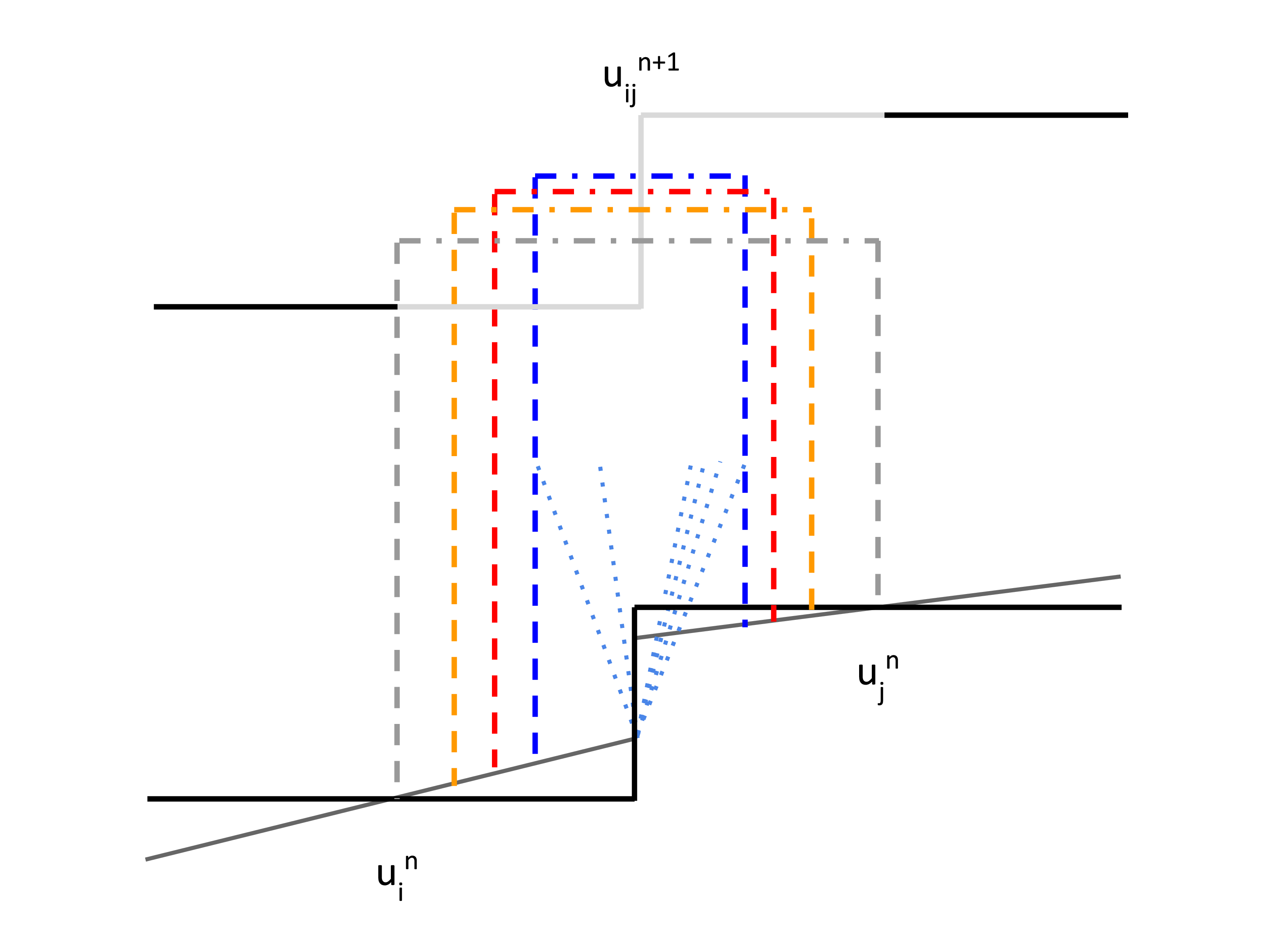
Figure 1: A schematic of a local Riemann problem between two particles \(u_{i}\) and \(u_{j}\), with the treatment of different numerical flux methods. Solid black lines represent the particle states at time \(n\), and solid dark grey lines represent a slope-limited gradient estimate. Dotted light blue lines are waves of the exact solution of the Riemann problem. Dashed grey lines represent the domain of dependence of the LxF scheme, notice that it influences a full half of both cells. Dashed orange lines represents the smaller domain of dependence of the KT scheme, at a distance of \(a\Delta{}t\) away from the interface. Dashed blue lines represents the domain of dependence using a Riemann solver. Dashed red lines represents the domain of dependence using the new switch, which is at most identical to the KT scheme for exactly colliding particles and lower anywhere else.
A schematic of this method in the context of two interacting particles and why this method is less diffusive is shown in Figure 1. From this, we see that we should expect diffusion to be decreased with this new switch, given that it limits the domain of dependence (determined by \(a\Delta{}t\)) to be less than or equal to that of the KT scheme. Here, diffusion occurs in the next step, where the middle state is projected back to the original particles via averaging - a larger domain of dependence means that the computed middle state is allowed to be more dominant in the averaging.
Implementation Details
We use the GIZMO code presented in Hopkins 2015 as the base for our implementation [3]. It includes various numerical methods, but we focus here on the two meshless schemes highlighted in [3]. Specifically, these are the original meshless discretization of Gaburov & Nitadori [2], Meshless Finite Volume (MFV), as well as the Meshless Finite Mass (MFM) scheme introduced in [3]. For these meshless methods, GIZMO employs both a gradient limiter as well as a pairwise slope limiter to project particle states to their interfaces during reconstruction, as detailed in Appendix B of [3]. To solve the local Riemann problems, it, by default, applies the approximate Riemann solver HLLC using Roe-averaged wave speeds.
We implement our methods by replacing just the Riemann solver with the numerical fluxes as computed by the KT scheme. We stress that the only component being changed is how numerical fluxes are computed – all other parts such as the meshless area approximations and both limiters are left unchanged. The inputs to replacement numerical flux schemes are the same interface states used as inputs to the Riemann solver.
Test Problems
Methods
We test six different methods: GIZMO-MFV, GIZMO-MFM, KT-MFV, KT-MFM, SWITCH-MFV, and SWITCH-MFM. The first two are the meshless methods presented in Hopkins 2015 which implement an approximate Riemann solver for its numerical flux computation [3]. Here, we use the unmodified, publicly-available version of GIZMO. The next two are implementations of the KT central schemes as a drop-in replacement for the Riemann solver in GIZMO. KT-MFV is the original formulation of the KT scheme, shown on Equation \ref{eq:KT_MFV} [1]. KT-MFM is the alternative finite-mass version where the particle interface moves with the contact wave, as given by Equation \ref{eq:KT_MFM}. The last two are identical to the KT schemes, except for the adjusted signal velocity on Equation \ref{eq:new_signal_velocity} with the switch on Equation \ref{eq:switch}.
Here, we compare the behaviour of the above six methods with a range of purely hydrodynamic tests. The KT scheme is more diffusive than the Riemann solver, as expected, but still captures the qualitative form of the solution, but with better stability properties. The switch behaves as intended, reducing diffusion in shearing tests, while being as accurate as the original KT scheme in shocktube problems. The MFM variant for each method follows the same trends when compared to the MFV variant of the same method, being in general more diffusive for most problems.
Shearing Flow
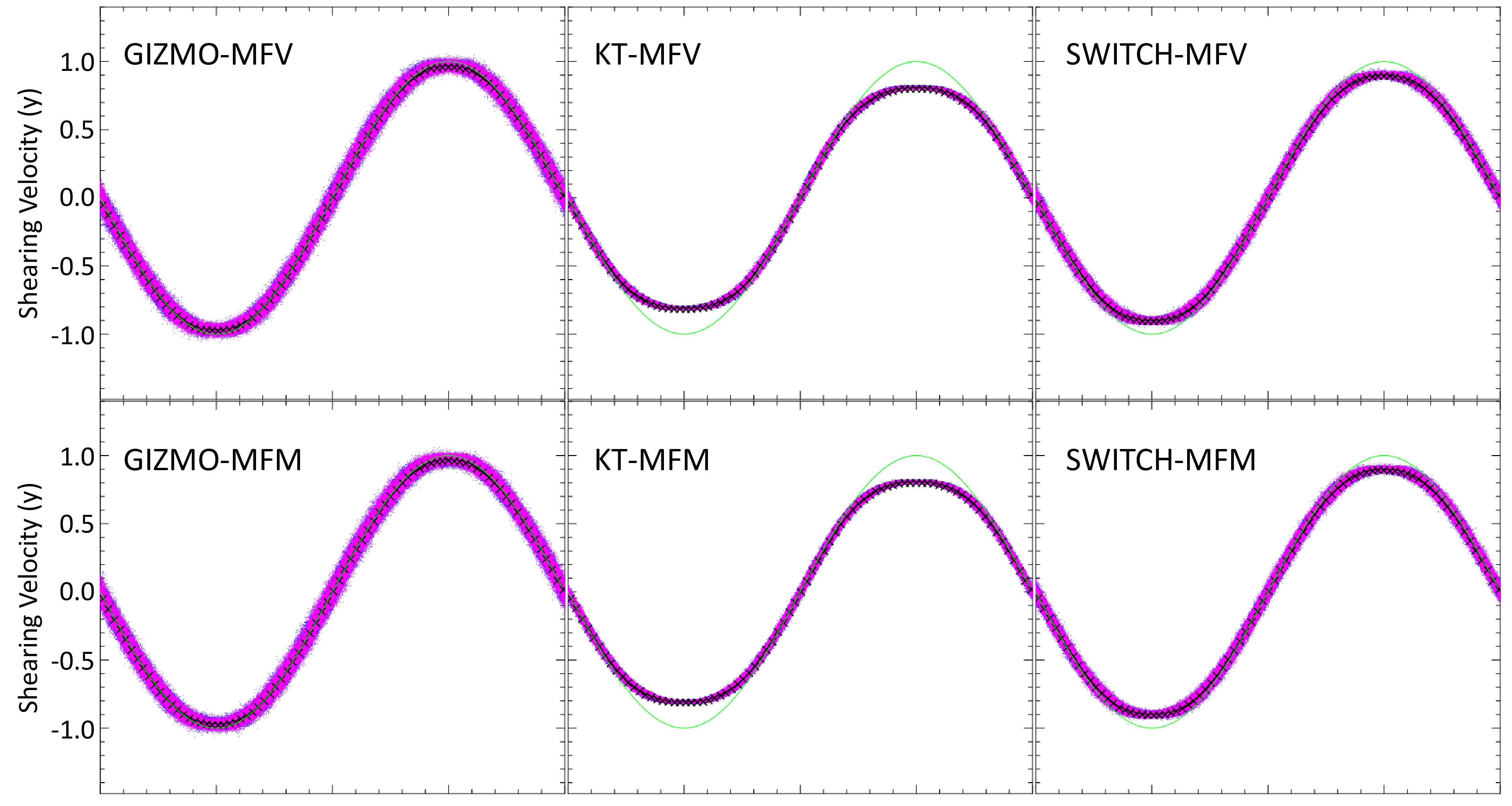
Figure 2: Shearing flow at \(t=5\), with particles represented as magenta dots and x’s representing binned particle averages, separated by one particle width. Notice that the peaks of the sine wave of the KT scheme are highly decayed, while the other methods approximately retain the original sinusoid (in green).
We begin with a relatively simple test to illustrate the problem with the KT scheme. We assume a homogeneous fluid with \(\rho=1\), \(e=1\), and a sinusoidal shaped shearing velocity in the y-direction, \(v_y = \sin(\pi{}x)\). This initial condition is a steady state, with no actual fluxes between particles. The particles should simply be advected. Thus, any change in state is solely a result of numerical diffusion. The shearing velocity profile at \(t=5\) is shown in Figure 2. Notice that the other methods remain very close to the original sinusoid, while there is noticable decay at the peaks in the KT scheme.
2D Gresho Vortex
As a more difficult test, we consider a \(C^1\) version of the triangular vortex by Gresho & Chan [16], where the points at \(r=0.2\) and \(r=0.4\) have been smoothed using piecewise parabolic functions. The azimuthal velocity is defined by,
\[\begin{align} v_{\phi}(r) = \begin{cases} 5r, & (0\leq{} r <0.16) \\ -62.5r^2+25r-1.6 & (0.16\leq{} r <0.24) \\ 2 - 5r & (0.24\leq{} r <0.36) \\ 31.25r^2 - 27.5r + 6.05 & (0.36\leq{} r <0.44) \\ 0 & (r > 0.44) \end{cases} \label{eq:greshovelocity} \end{align}\]and the pressure by,
\[\begin{align} P(r) = \begin{cases} \frac{25}{2}r^2 & (0\leq{} r <0.16) \\ \frac{15625}{4}r^4 - \frac{3125}{3}r^3 + \frac{825}{2}r^2 - 80r + 2.56\ln(\frac{r}{0.16}) + \frac{464}{75} & (0.16\leq{} r <0.24) \\ \frac{25}{2}r^2 - 20r + 4\ln(r) + 2.56\ln(1.5) - 4\ln(0.24) + \frac{11}{3} & (0.24\leq{} r <0.36) \\ \frac{976.563}{4}r^4 - \frac{1718.75}{3}r^3 + \frac{1134.38}{2}r^2 - 332.75r + 36.6025\ln(r) \\ \quad\quad + 6.56\ln(1.5) - 36.6025\ln(0.36) + 77.13154890048 - \frac{152}{15} & (0.36\leq{} r <0.44) \\ 49.6801625856 - \frac{176.81}{3} + 36.6025\ln(\frac{11}{9}) + 6.56\ln(\frac{3}{2}) & (r > 0.44) \end{cases} \label{eq:greshopressure} \end{align}\]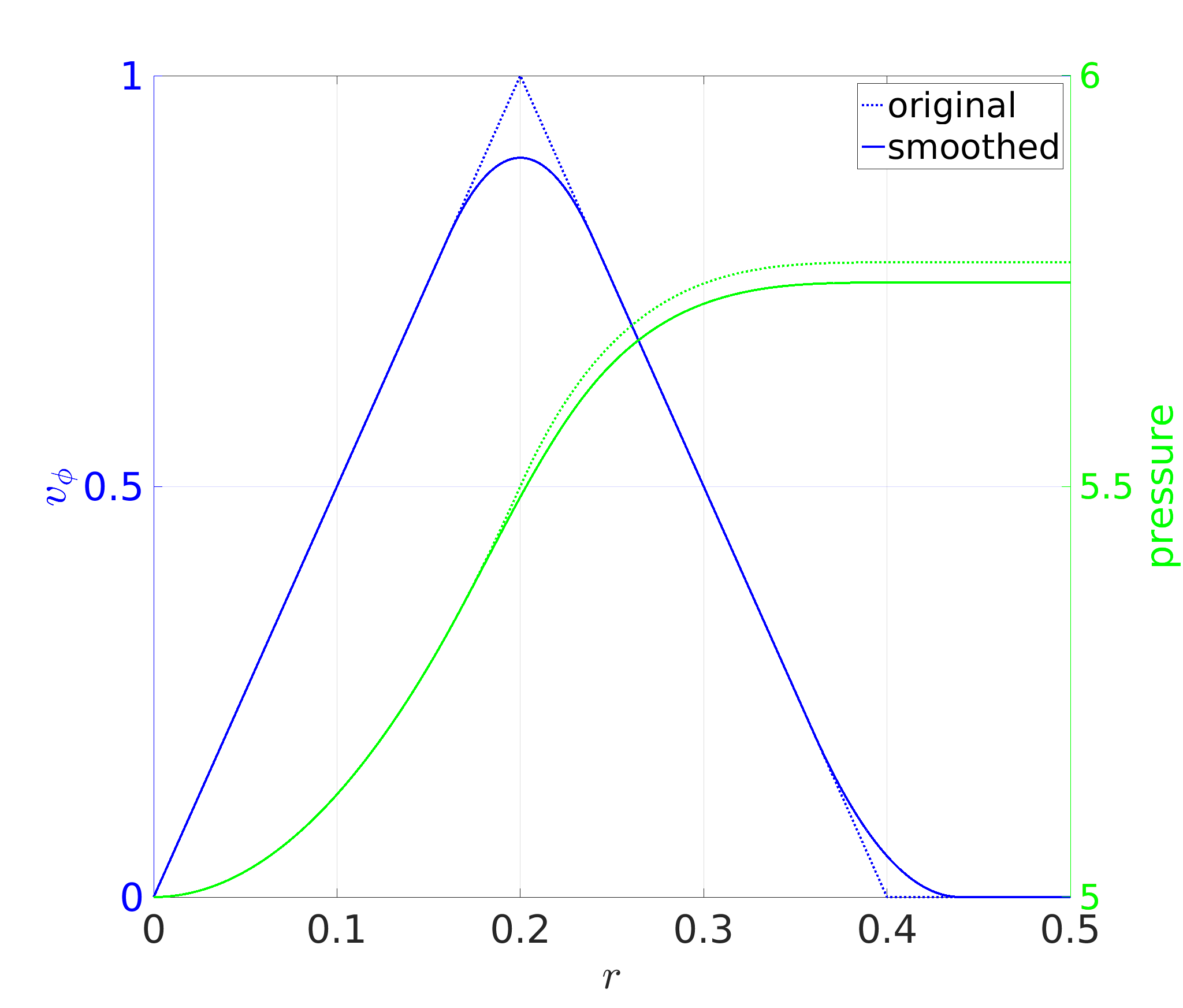
Figure 3: The initial condition of the Gresho-Chan vortex, for both the \(C^1\) (labelled smoothed) version as well as the original piecewise linear version from Gresho & Chan 1990 [16]. The left (blue) axis shows the azimuthal velocity profile and the right (green) axis shows the pressure profile that exactly cancels out the rotational force to produce a steady-state solution.
and zero radial velocity. The velocity and pressure profiles of the \(C^1\) version compared to the original are shown in Figure 3. This test was performed in 2D using particles initially distributed in a regular grid, and a simulation domain of \([-1,1]\times[-1,1]\) to allow the vortex space to decay without influencing itself through the periodic boundary conditions.
This setup is a steady-state solution, where the rotational force is exactly cancelled out by the pressure gradient. While the inner portion (\(x<0.2\)) is in rigid body rotation and is relatively easy to simulate accurately, the outer region of the vortex has particles shearing against each other as the inner particles rotate with a faster angular velocity than the outer particles. Since there should be no mass or momentum transfer radially, this setup allows us to assess the amount of numerical diffusion required, with deviations from the steady-state solution being known to be due to excessive numerical diffusion.
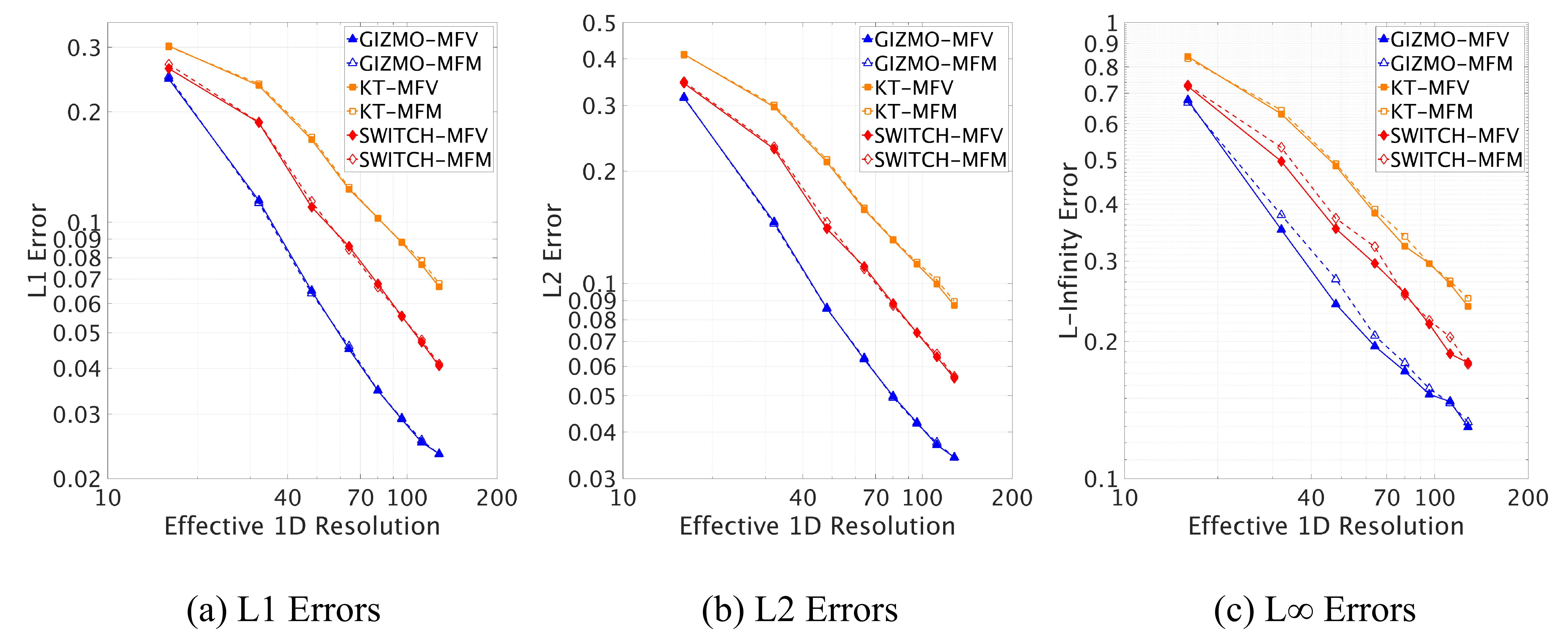
Figure 4: Error norms for the azimuthal velocity of the Gresho-Chan vortex using different methods in 2D. Norms were computed for particles within \(r<0.5\) at \(t=3.0\) on a log-log plot against the effective \(1D\) resolution. Initial conditions have an effective \(1D\) resolutions of multiples of \(16\), up to \(128\).
We can quantitatively measure the error of the solution through various norms, which can be used to look at the convergence of each method. We choose to plot the \(l_1\), \(l_2\), and \(l_\infty\) error norms of the azimuthal velocity for particles within \(r<0.5\) at time \(t=3.0\), which are shown in Figure 4, with convergence rates shown on Table 1. We see that convergence for this problem is approximately linear in \(L1\) and \(L2\). This matches results from Hopkins 2015 for GIZMO [3], as well as other existing results for particle-based methods [17]. We see that in all three norms, the Riemann solver methods have the best convergence rates as well as smaller errors in general. We emphasize the degree to which the switch improves on the KT scheme, especially in convergence. The convergence rates of the SWITCH methods are much closer to the rates of the Riemann solver methods, and is actually better when measured in the \(L_\infty\) norm. The \(L_\infty\) result is due to reduced noise, which is not surprising for a more diffusive method.
Table 1: Convergence rates for the Gresho-Chan vortex in 2D computed within \(r<0.5\) on \(t=3.0\).
| GIZMO-MFV | GIZMO-MFM | KT-MFV | KT-MFM | Switch-MFV | Switch-MFM | |
|---|---|---|---|---|---|---|
| L1 | -1.1608 | -1.1448 | -0.9098 | -0.9046 | -1.0776 | -1.0806 |
| L2 | -1.0487 | -1.0401 | -0.8837 | -0.8747 | -1.0013 | -1.0107 |
| L\(\infty\) | -0.6890 | -0.7561 | -0.6988 | -0.6909 | -0.7390 | -0.7763 |
3D Gresho Vortex
We repeat the above Gresho Vortex setup (Equations \ref{eq:greshovelocity} and \ref{eq:greshopressure}) in 3D with a glassy initial particle distribution and a simulation domain of \([-1,1]\times[-1,1]\times[-0.5,0.5]\). A glassy distribution means the particles are arranged in no particular order, but enforcing a near-constant nearest neighbour distance for all particles. In this way, we avoid dominant axes but keep a near-uniform particle density.
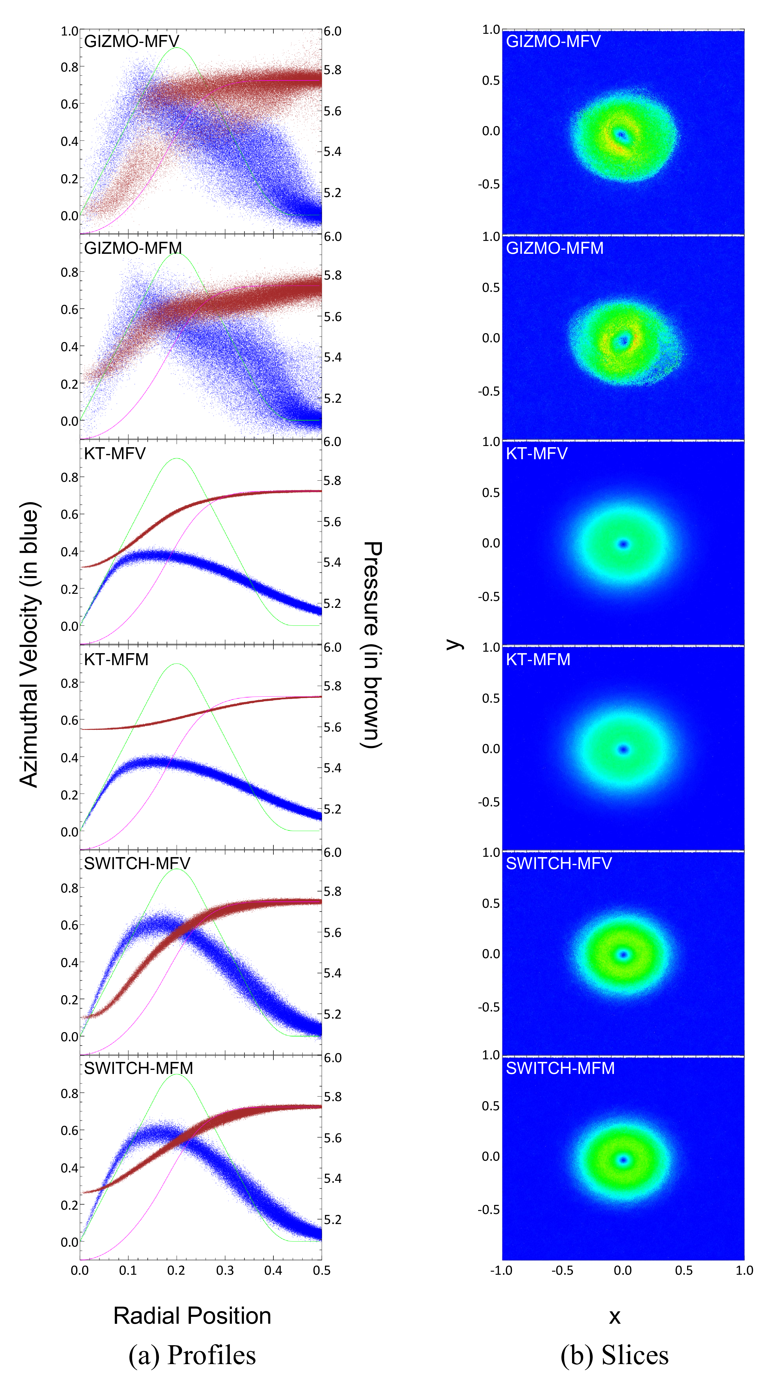
Figure 5: Results for the smoothed Gresho Vortex with an effective 1D resolution of \(64\). (a) Azimuthal velocity profiles (blue points) and pressure profiles (brown points) for numerical solutions of the Gresho-Chan vortex at \(t=4.0\) (\(\approx{}2.9\) rotations). Exact steady-state solution is shown as green lines for velocity and magenta lines for pressure. (b) Velocity slice coloured from blue (\(v_\phi = 0\)) to red (\(v_\phi = 1\)).
The results for an effective 1D resolution (i.e. the inverse of the average particle separation) of \(64\) are shown in Figure 5. We see that while the azimuthal velocity for the KT scheme is almost nearly wiped out at \(t=4\), the inclusion of the new switch better preserves the structure of the vortex, albeit with a small negative impact on the particle deviation. This small increase in noise is an expected tradeoff of reducing the amount of diffusion applied, given that diffusion inherently smooths small scale local deviations. Also notice that, due to the diffusive conversion of kinetic to potential energy, the pressure for the KT scheme rises at the center, whereas the switch reduces this increase.
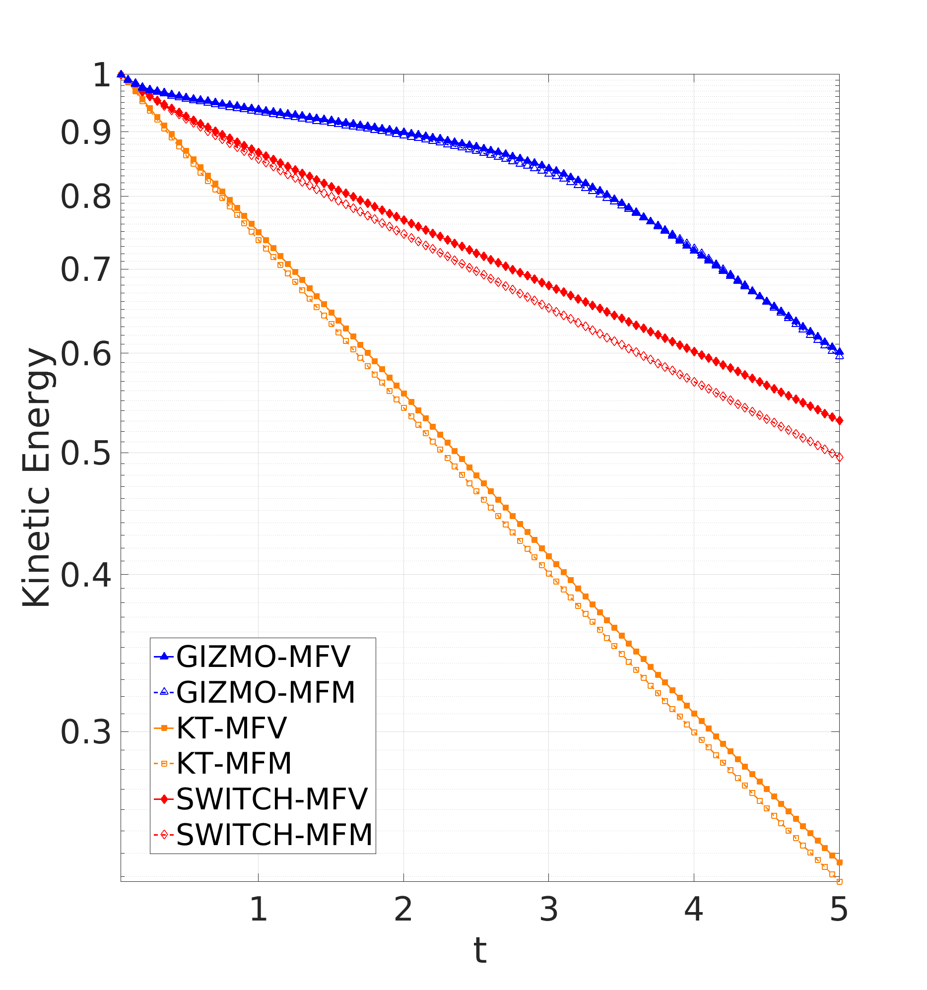
Figure 6: Kinetic energy over time of the Gresho-Chan vortex on a semilog plot, normalized by the initial kinetic energy. Notice the clear change in behaviour for the GIZMO-MFV and GIZMO-MFM schemes at around \(t=3\), due to an instability forming.
On the other hand, the Riemann solver schemes retain the original structure for longer, but quickly deviate from the steady state solution around \(t=3\) via a non-physical instability. This numerical instability is likely seeded by small (grid-scale) particle noise from the glassy initial condition, and demonstrates a pitfall in applying too little diffusion. The particle noise should be dominated by the physical structure, especially given that the smoothed initial condition already aids in preventing numerical instability by allowing the gradient of the velocity and pressure to change over several particles, rather than instantaneously in a sub-resolution scale. Longer simulations showed that KT and SWITCH never developed such structure, and evenly dissipate energy until the velocity is uniformly zero. This time-dependent behaviour is shown in Figure 6, where we see that both KT and SWITCH have a consistent exponentially decaying kinetic energy, while the other three schemes transition from a very slow initial decay to a very rapid decay as an instability forms. Here, we also see the extra diffusion in the MFM variants compared to MFV, with the kinetic energy decaying faster.
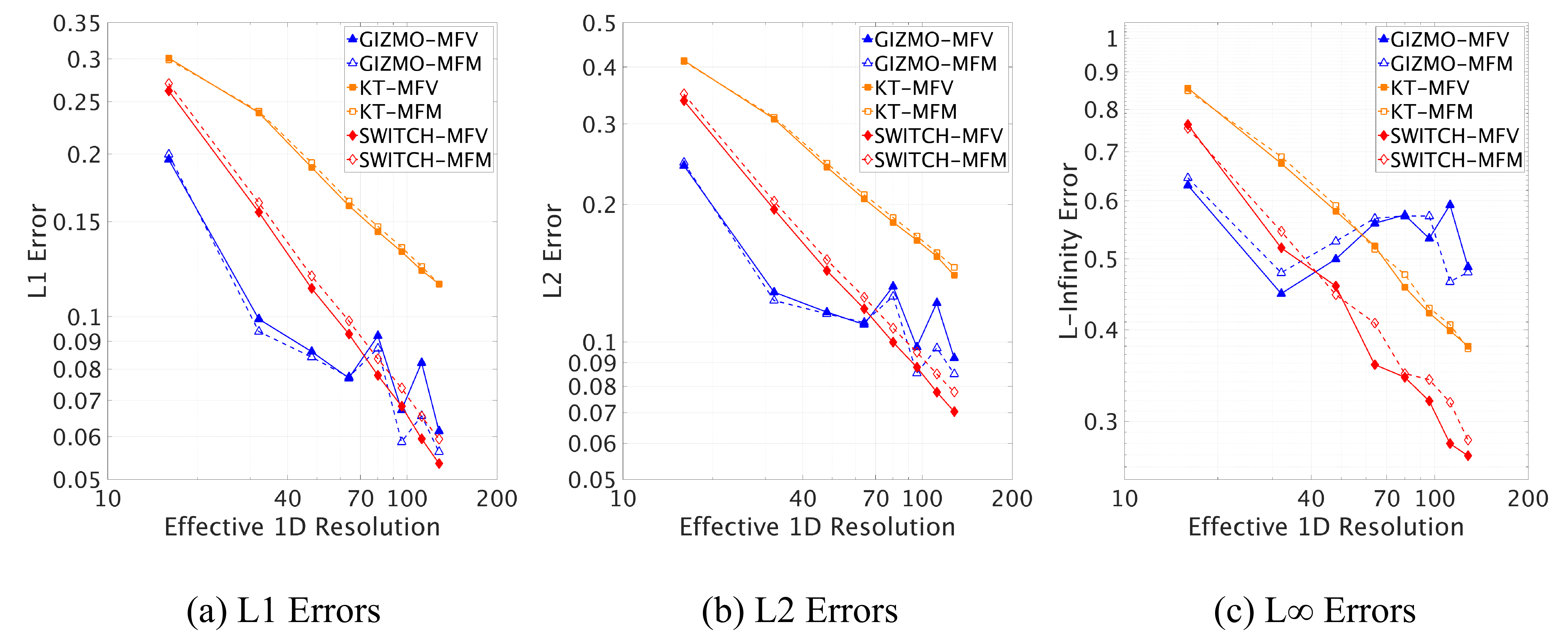
Figure 7: Error norms for the azimuthal velocity of the Gresho-Chan vortex using different methods in 3D. Norms were computed for particles within \(r<0.5\) at \(t=3.0\) on a log-log plot against the effective \(1D\) resolution. Initial conditions have an effective \(1D\) resolutions of multiples of \(16\), up to \(128\).
We once again plot the three error norms against resolution, shown in Figure 7. We see that in general, the Riemann solver is more accurate than KT and SWITCH, but that KT and SWITCH methods are better converged. In the \(l_1\) and \(l_2\) norms, the errors of the Riemann solver methods do not decrease following some power law, but erratically increases and decreases as a result of the unpredictable formation of secondary structures seeded by particle noise. This is less so the case in lower resolutions, which are too coarse to allow the formation of secondary structures, meaning the physical vortex remains dominant. In a sense, the secondary structures formed in GIZMO-MFV and GIZMO-MFM are of a fixed resolution, and at lower resolutions it simply is absorbed into the actual physical structure. This is also shown in later tests. Even more interestingly, the \(l_\infty\) norm of GIZMO-MFV and GIZMO-MFM methods do not converge at all, suggesting that there are always at least a few particles in an ill-conditioned situation due to particle noise. We would thus like to stress the value of a method that reliably diffuses away grid-scale noise rather than evolving them physically.
Fitting a power law gives the convergence rates shown on Table 2. From this, we see that the SWITCH methods have the best convergence rates, with around \(N^{-0.75}_{1D}\), though all methods converge sublinearly – showing increased difficulty with the added degree of freedom in 3D. We once again wish to point out the degree to which the switch improved the convergence rate of the KT scheme, jumping from a similar rate to GIZMO-MFV and GIZMO-MFM, to well above. The switch converges so well that it rivals the solution of the Riemann-solver based methods at \(N_{1D} = 64\).
Table 2: Convergence rates for the Gresho-Chan vortex in 3D computed within \(r<0.5\) on \(t=3.0\).
| GIZMO-MFV | GIZMO-MFM | KT-MFV | KT-MFM | Switch-MFV | Switch-MFM | |
|---|---|---|---|---|---|---|
| L1 | -0.441 | -0.532 | -0.480 | -0.466 | -0.756 | -0.726 |
| L2 | -0.348 | -0.439 | -0.518 | -0.504 | -0.748 | -0.720 |
| L\(\infty\) | 0.003 | -0.069 | -0.398 | -0.386 | -0.498 | -0.446 |
Colliding Flows Shocktube
To demonstrate that the new scheme still applies the appropriate amount of diffusion to safely smooth discontinuities, we consider a simple 1-dimensional Riemann problem representing two flows colliding with a constant velocity. We use a homogeneous initial fluid, with \(\rho=0.125\) and \(P=0.05\), differing only in fluid velocity between two fluid domains:
\[\begin{align} v_x = \begin{cases} 1.0 & x<0 \\ -1.0 & x>0 \end{cases} \end{align}\]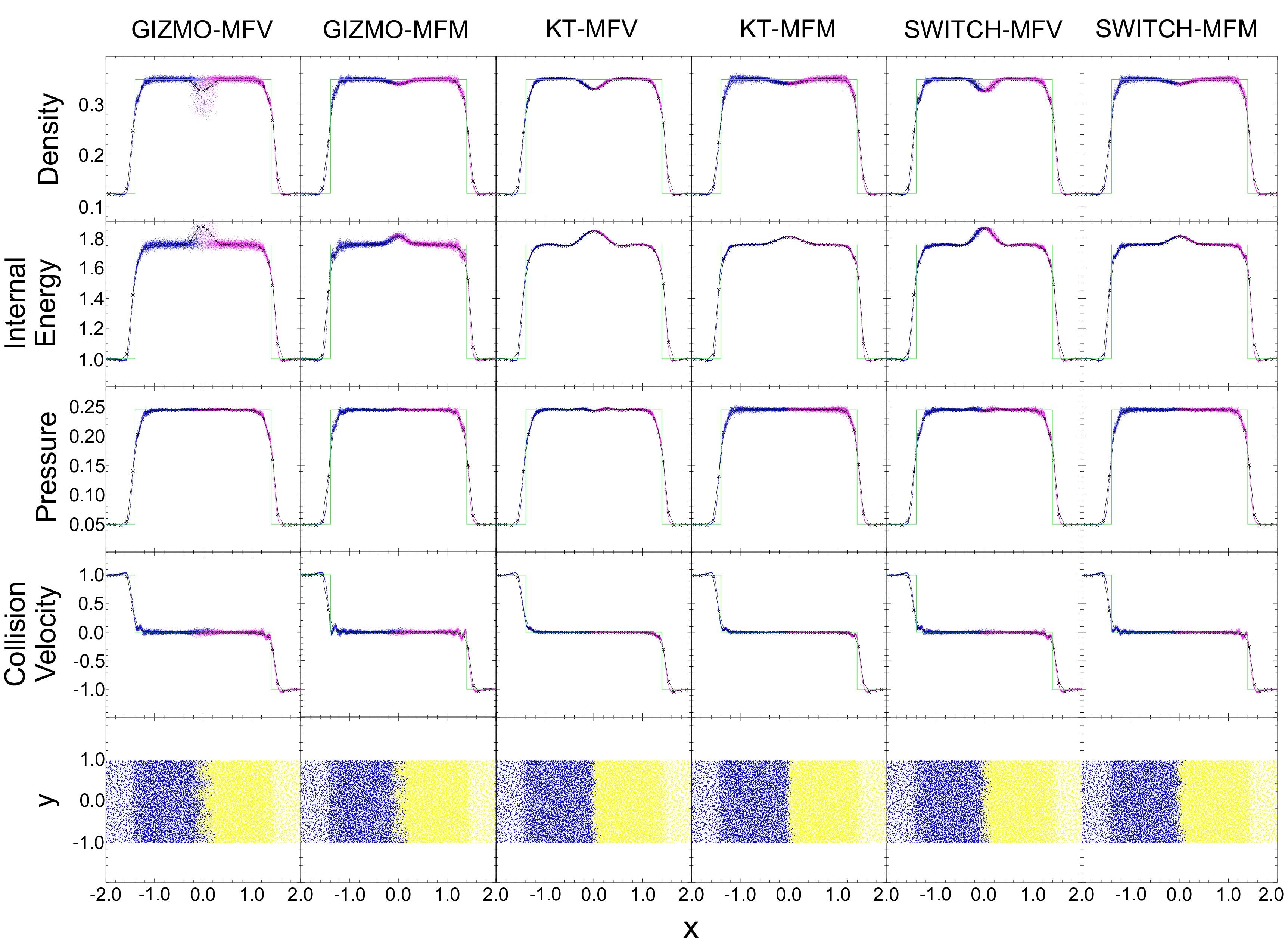
Figure 8: Results for the colliding flows test at \(t=2.5\). From top to bottom, mass density, internal energy, pressure, collision velocity (\(v_x\)), and z-projected slice. The black line represents binned averages of the numerical solution, with x’s separated by effective 1-dimensional resolution. The green line represents the analytic solution. In the upper four rows, blue points represent particles originally in \(x<0\) and magenta points represent particles originally in \(x>0\). In the last row, blue points represent particles originally in \(x<0\) and yellow points represent particles originally in \(x>0\).
This generates two outwards-moving shocks with the horizontal velocity completely cancelling in the post-shock region. We simulate this using a 3-dimensional glassy initial condition with constant particle masses, with results shown in Figure 8.
As shown, all methods are able to capture the discontinuity by smoothing the shocks over about three particles. In general, the more diffusive methods have less particle dispersion, less post-shock ringing, and less particle inter-penetration. As previously noted, higher diffusivity reduces dispersion by smoothing out local variability. With regards to the difference between KT and SWITCH methods, the increased dispersion comes from reduced diffusion along the y- and z-axes, allowing particles located laterally to have larger differences in fluid properties.
Higher diffusivity also reduces particle inter-penetration as particles near the boundary at the beginning of the simulation are able to convert their kinetic energy into heat faster via the diffusive mechanism. Looking at the slices, the penetration is inhomogeneous: in certain regions the left fluid penetrates further and others, the right fluid penetrates further. This suggests that the inhomogeneity is seeded by particle noise in the initial condition, which the less diffusive methods interpret as possible instability. Post-shock ringing does not satisfy the TVD condition, and is a symptom of insufficient diffusion to maintain stability. Only the KT scheme, which was previously shown to satisfy a sufficient condition for TVD, has no noticable oscillation, while the rest have in varying degrees.
The majority of the error in this colliding flows test occurs at the initial collision interface (\(x=0\)), and is a consequence of the well-known wall-heating problem [18]. Wall-heating stems from the rapid conversion of kinetic energy into thermal energy at the collision interface. Since the momentum equations find the correct pressure as the shock forms, the density is forced to fall; lack of conduction keeps error in the energy local. Noh 1987 showed this heating is purely a consequence of numerical diffusion [18], and it is shown later that this leads to nonuniform convergence for the inviscid problem, as higher resolutions decreases the width of the wall heating, but not its magnitude [19].
Interestingly, the MFM variants suffer less than MFV from wall heating. For KT and SWITCH, the MFM variants have slightly larger density noise, stemming from not being able to diffuse away density variations due to the enforced particle masses.
Shearing Shock
Next, we consider a test where the fluid has both shock and shear characteristics. This test is important for validating the new switch, which controls diffusion depending on the relative amount of shocking and shearing of the fluid locally. We consider a shocktube setup similar to that used in Section 7.4, with the same uniform density and pressure. In addition to a colliding x-component of the velocity, we add opposing y-components to produce a transverse velocity jump across the interface:
\[\begin{align} v_x &= \begin{cases} -\delta{}_x & x<0 \\ \delta{}_x & x>0 \end{cases} \\ v_y &= \begin{cases} \delta{}_y & x>0 \\ -\delta{}_y & x>0 \end{cases} \end{align}\]The magnitudes \(\delta{}_x\), \(\delta{}_y\) are varied to test fluids with different proportions of shock and shear. The solution involves a complete cancellation of the x-component velocity in the postshock region, leaving a pure shear flow. Ideally, the addition of the switch should not adversely affect the performance of the method as the flow transitions from a pure shock to a pure shear. We expect the SWITCH methods to be slightly worse for a pure shock, due to a slight increase in noise seen in Figure 8, but better for a pure shear where the reduced diffusion truly applies.
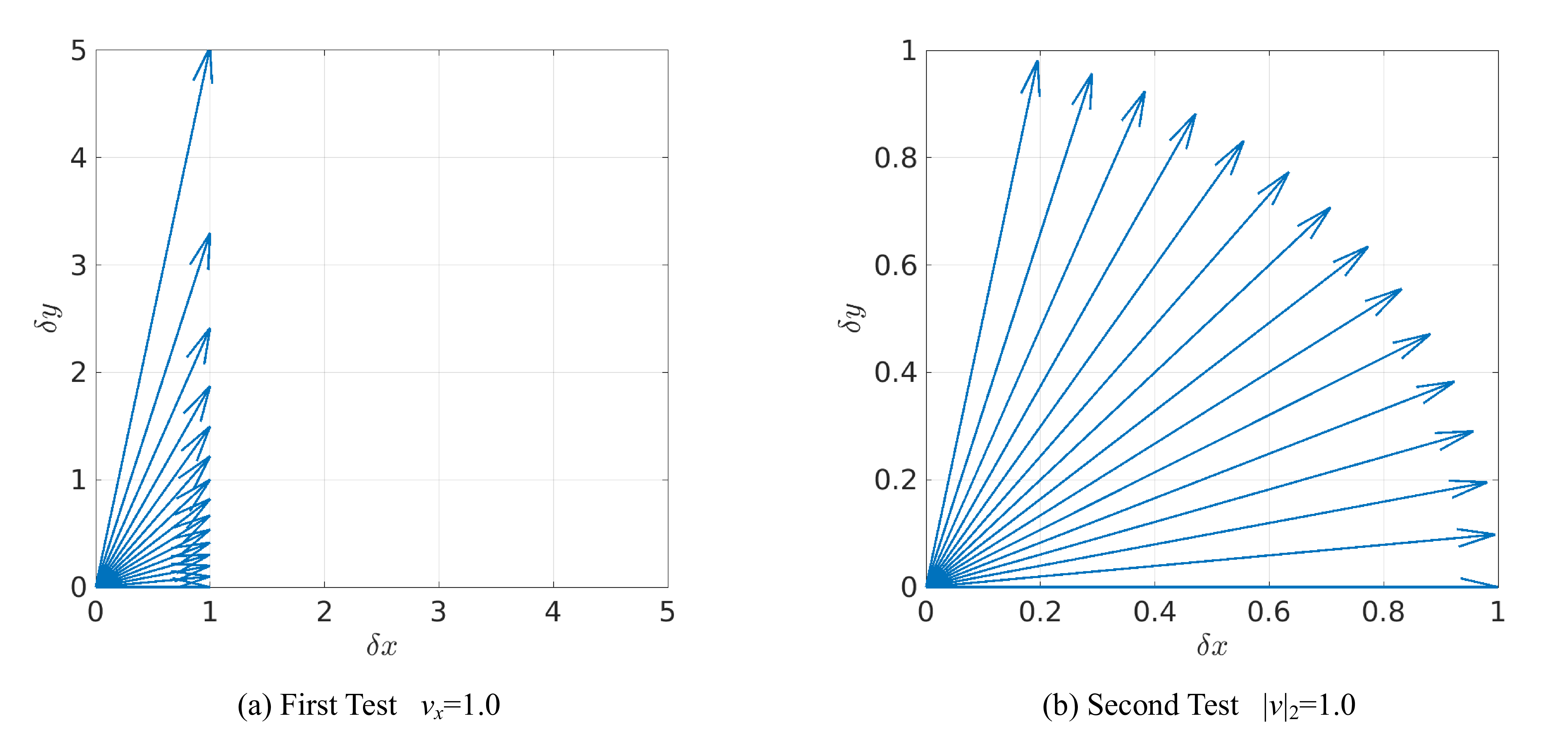
Figure 9: \((\delta{}_x,\delta{}_y)\) used for the two tests stated in Section 7.5
We test two variants of this problem. We let \(\theta\) be the angle between \((1,0)\) (representative of the normal of the interface) to a velocity vector \((\delta{}_x,\delta{}_y)\). In both tests, we use angles \(\theta\in[0,14\pi/32]\) of multiples of \(\pi/32\). For the first test, we hold constant \(\delta{}_x = 1\) and vary \(\delta{}_y\) to get \(\theta\), while for the second test we hold constant the magnitude \(\|(\delta{}_x,\delta{}_y)\|_2 = 1\) and vary both \(\delta{}_x\) and \(\delta{}_y\). The entire set of velocities used for both tests are shown in Figure 9. Angles \(15\pi/32\) and \(\pi/2\) were avoided since the first test would involve infinitely large \(\delta{}_y\).
The \(l_1\) errors are shown in Figure 10. Overall, we find that the switch behaves well even in regimes between shocks and shears. Since this is a variant of the above colliding flows problem, the error - especially for the first test - is dominated by wall heating. This is apparent when comparing the MFV and MFM variants, where the MFM variants having less error due to the reduced wall heating. We also note that because the Riemann problem (as formulated in GIZMO) is Galilean invariant, the only difference between this problem and the non-shearing problem is during the formation of the shock, when particles initially collide. The propagation of the shock is identical for all tests, since the y-component of velocity is constant across the shock and thus irrelevant in the rest frame of the particle pair interface. This further indicates that errors remain localized around \(x=0\).
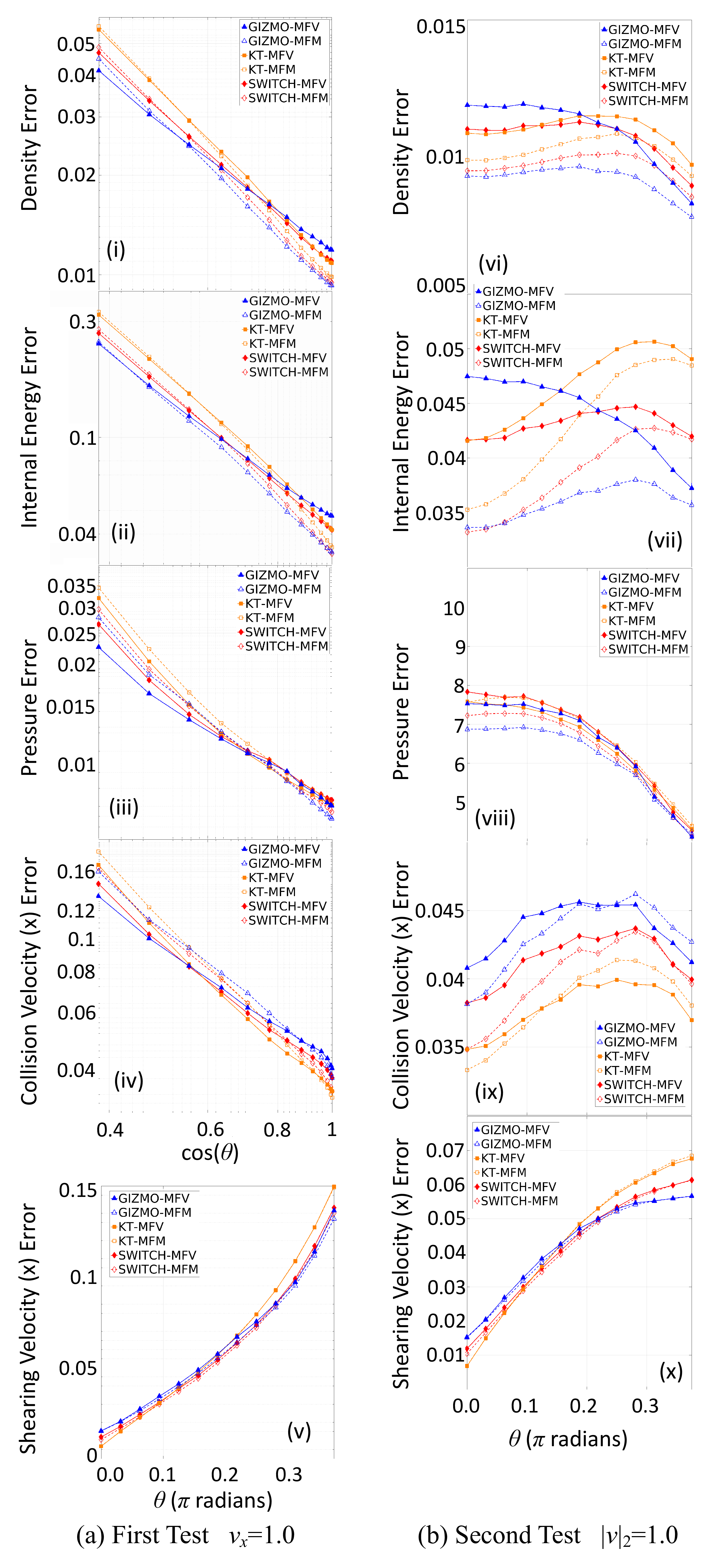
Figure 10: \(L1\) Error norm for the two shearing shocktube problems. (a) The first shearing shocktube problem has \(v_x = 1.0\), with \(v_y\) being varied so as to produce \(\theta \in{}[0,14\pi/32]\) of multiples of \(\pi/32\). Here, the first four variables (i)-(iv) are shown in a log-log plot against \(\cos(\theta)\) to better represent the expected dependency. (b) The second shearing shocktube problem has \(\|v\|_2 = 1.0\), with both \(v_x\) and \(v_y\) being varied so as to produce \(\theta \in{}[0,14\pi/32]\) of multiples of \(\pi/32\). The \(L1\) norm was computed for \(x\in[-2,2]\).
Noh 1987 shows that the wall heating error is dependent on the amount of numerical diffusion applied [18]. For the KT and SWITCH methods, numerical diffusion is proportional to the wave propagation speed, \(a\). Since the sound speed, \(c\), remains constant in this problem, we expect numerical diffusion to be proportional to \(\|\mathbf{v}\|_2\) alone. For the first test, \(\|\mathbf{v}\|_2=1/\cos(\theta)\), while for the second, \(\|\mathbf{v}\|_2=1\). As shown by Figure 10, we get close to the expected result of the errors being \(\propto{}(\cos(\theta))^{-1}\) for the first test and near constant for the second. The power law slope of the L1 and L2 errors in density are shown on Table 3. We see the power law fits are slightly steeper than the expected \(\cos(\theta)^{-1}\), in both norms. A more rigorous error analysis could be used to explain why this is the case, but is unnecessary for the purpose of validating the new switch.
Table 3: Power-law fits for the errors in density of the first version of the shearing shock test at \(t=2.5\).
| GIZMO-MFV | GIZMO-MFM | KT-MFV | KT-MFM | Switch-MFV | Switch-MFM | |
|---|---|---|---|---|---|---|
| L1 | -1.321 | -1.613 | -1.597 | -1.685 | -1.485 | -1.630 |
| L2 | -1.043 | -1.251 | -1.218 | -1.318 | -1.146 | -1.275 |
We now examine on how the switch behaves relative to the other methods. As expected, in density and internal energy – the variables directly affected wall heating – SWITCH is very similar to the usual KT scheme for small \(\theta\), but has smaller error in more shear-like flows. This trend is matched in other variables for the constant-\(\delta{}_x\) test. The second test is perhaps more indicative of the behaviour of the methods, as it removes the increasing velocity magnitude – and thus increased wall heating – as the angle is increased. The advantage of the switch is clearly shown in density and internal energy - it once again matches the error for small \(\theta\), but has significantly less error for shearing flows. The switch produces slightly worse in pressure, although this error is very small in magnitude and is primarily due to noise. The switch has larger errors in collision velocity due to stronger post-shock ringing, but better for the shearing velocity. The unnecessary diffusion of the shear component in the KT scheme is clear from the shearing velocity error, which is strongly dependent on the angle; note that all methods increase in error since the magnitudes of the y-velocities themselves increase according to angle.
Kelvin-Helmholtz Instability
Finally we consider the Kelvin-Helmholtz (KH) instability, which occurs when a shearing flow is slightly perturbed, causing an evolution of waves into vortices [8]. This example tests how the methods handle the generation of mixing and turbulence via a dynamic instability. We use the setup from McNally et. al. [20], where a \(1\times{}1\times{}0.125\) periodic box is separated into two halves in equilibrium with properties:
\[\begin{align} \rho &= \begin{cases} 2 & y\in (-0.25, 0.25) \\ 1 & otherwise \end{cases} \\ e &= \begin{cases} 1.875 & y\in (-0.25, 0.25) \\ 3.75 & otherwise \end{cases} \end{align}\]The shear is defined by:
\[\begin{align} v_x = \begin{cases} -0.5 + 0.5e^{(y+0.25)/L} & y\in[-0.5,-0.25) \\ 0.5 - 0.5e^{(-0.25-y)/L} & y\in[-0.25,0) \\ 0.5 - 0.5e^{(y-0.25)/L} & y\in[0,0.25] \\ -0.5 + 0.5e^{(0.25-y)/L} & y\in[0.25,0.5) \end{cases} \end{align}\]where \(L\) is a smoothing parameter. We choose to use both a thin shear interface \(L=0.00625\) and a thicker shear interface \(L=0.025\) – at the resolution used, the shear transition occurs along \(4\) particles for the former and \(16\) for the latter. The instability is seeded by a vertical velocity perturbation to the interface:
\[\begin{align} v_y = 0.01\sin(4\pi{}x) \end{align}\]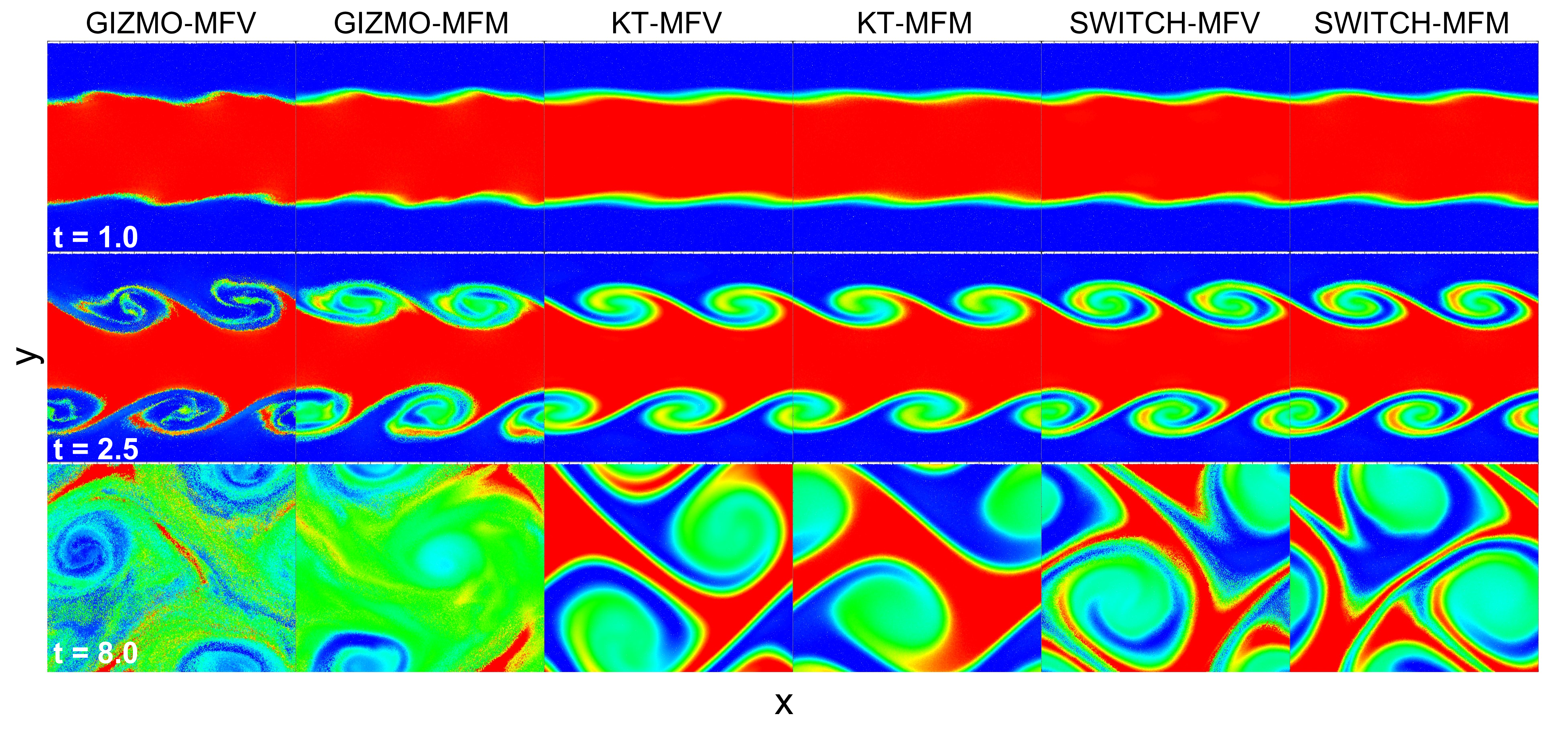
Figure 11: Density slice for the Kelvin-Helmholtz instability with a thick interface (16 particle widths). Red represents a density of \(2\), and blue represents a density of \(1\).
Once again, we use a glassy initial particle distribution, with constant particle masses such that the number density of particles is doubled for the middle band. The box resolution is \(192\times{}128\times{}16\) particles. Density slices for times \(t=1\), \(t=2.5\), and \(t=8\) are shown in Figure 11 for the thick shear transition, and Figure 12 for the thinner transition.
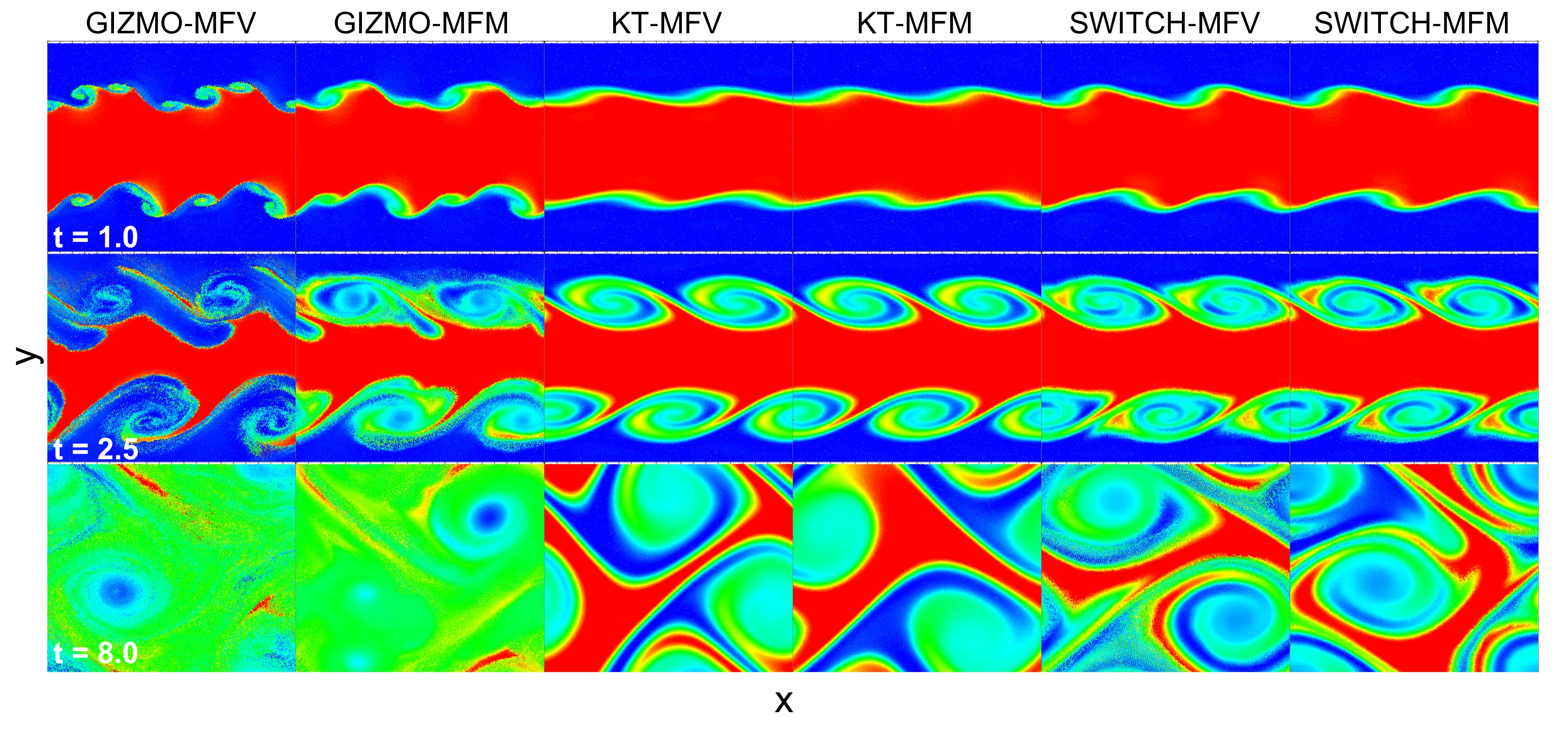
Figure 12: Density slice for the Kelvin-Helmholtz instability with a thin interface (4 particle widths). Red represents a density of \(2\), and blue represents a density of \(1\).
The reduction of diffusion provided by the switch allows it to capture slightly more vortices than the original KT scheme in both cases. Additionally, we note that even at the longer time \(t=8\), the overall structure with the switch does not greatly vary from that without the switch, unlike the result of GIZMO-MFV and GIZMO-MFM. We see from the \(t=1\) result for the thin transition test, that the Riemann solver methods qualitatively do not agree with the other four methods – the vortices produced are distorted. This is likely caused by particle noise in the initial condition. The more diffusive KT and SWITCH schemes are able to damp this grid-scale noise, while the Riemann solver methods treat it is a physical small-wavelength mode in the KH problem. Such small-wavelength modes thus generate smaller scale vortices which distort the KH vortices. This is confirmed by tests with smaller box resolutions, where unphysical smaller vortices did not develop, suggesting that the grid-scale modes seeded by particle noise could not develop faster than the KH vortices. Additionally, we note that this increased mixing causes the mode amplitude to be much larger than with the other two methods.
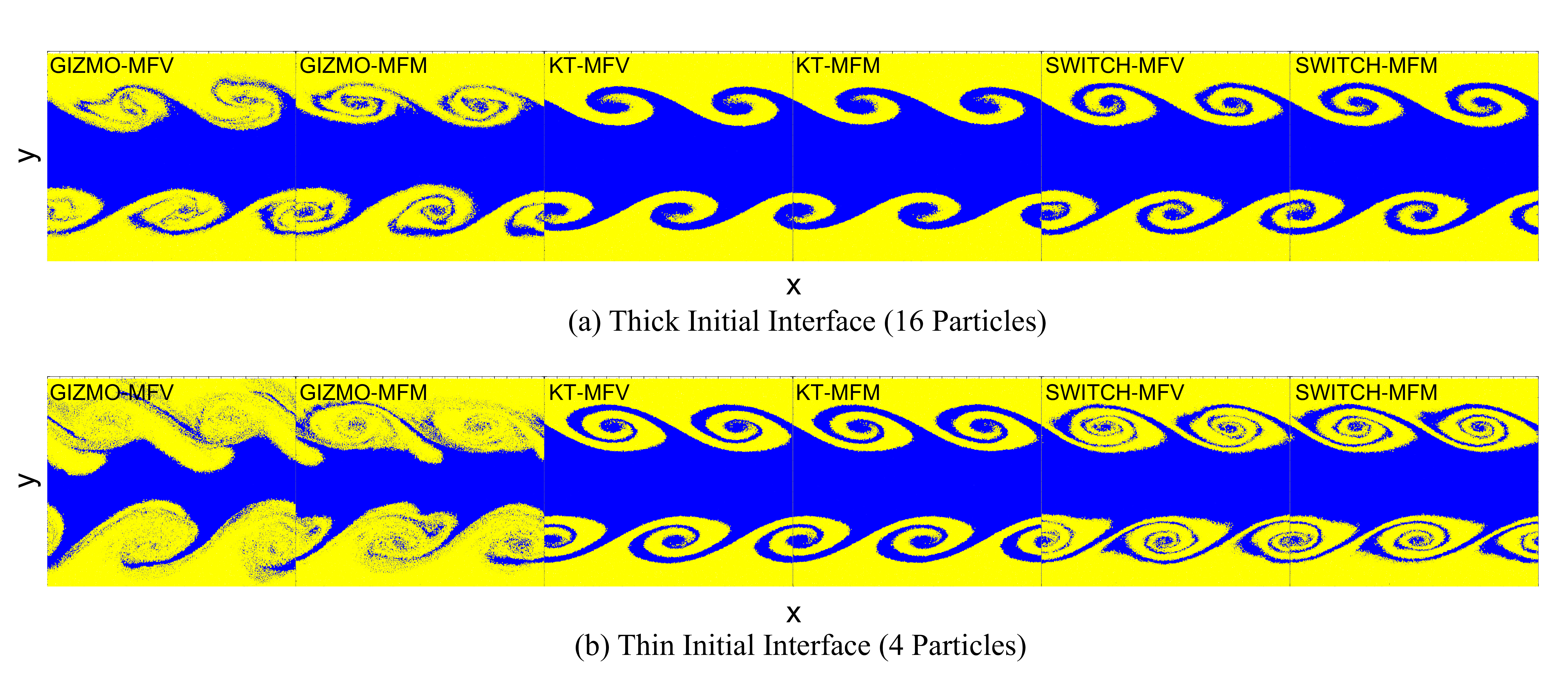
Figure 13: Slice of the KH instability at \(t=2.5\) for both the (a) thick initial interface and (b) thin initial interface, coloured by the initial particle locations. Blue represents particles initially in the high density middle band, and yellow represents particles originally in the low density upper and lower bands.
Agreement of Riemann solver methods is closer when the transition width is increased to \(16\) particles, although it still greatly deviates at long time. Even in this case, grid-scale noice causes formation of smaller vortices just before before the velocity-seeded vortices. The increased interface width, however, causes difficulty for the KT and SWITCH methods, with the vortices evolving thicker and more blurred. It is apparent that even with the switch, there is still much shearing diffusion allowed to occur, thickening the interface. In this case, however, the diffusion is largely limited to density. Plotting a slice coloured based on the origin of the particles as shown in Figure 13, we find that the switch allows the vortices to develop much further, but the structure is obscured by diffusion in density. As well, we see that the Riemann solver methods suffer greatly from particle penetration (i.e. mixing) in the vortices, with the two phases of the fluid starting to become homogeneous. It may be possible to choose a different, more aggressive switch on the density to further limit the amount of diffusion but maintain good behaviour in momentum and energy.
Lastly, we note that for KT and SWITCH, the difference between MFV and MFM variants are very minor, with MFV forming slightly more defined vortices than MFM. One notable difference, however, is that SWITCH-MFM greatly reduces particle inter-penetration, especially at later time. The Riemann solver methods, MFV and MFM, produce drastically different results, with MFV characterized by more sharply defined shear boundaries than MFM. The sharp boundary for GIZMO-MFV demonstrates the effectiveness of the meshless method to mimic moving-meshes where the boundary would be sharply defined by the mesh boundaries. Here, however, it simply fails to provide enough diffusion to damp unintended grid-scale noise, leading to rapid growth of small wavelength modes that destroy the intended vortices.
It is possible to consider the Riemann solver methods here to be more accurate, under the interpretation that grid-scale noise in the initial condition should be resolved and allowed to generate small scale vortices. We argue, however, that such susceptibility to grid-scale noise is undesirable for numerical methods since grid scale fluctuations are, by definition, poorly resolved and unlikely to be physically significant.
Computational Cost
Table 4: Wallclock time for the shearing flow problem (Section 7.1) and the \(\theta=0\) shocktube problem (Section 7.4). The CPU used is an AMD R7 1700 in both cases, using 8 cores for the shearing flow problem and 1 core for the shocktube. The shearing flow was progressed to \(t=5\), while the shocktube was progressed to \(t=0.5\).
| Shearing Flow | Shocktube | |
|---|---|---|
| GIZMO-MFV | 539m26s | 3m16.02s |
| GIZMO-MFM | 521m41s | 3m8.80s |
| KT-MFV | 548m15s | 3m15.26s |
| KT-MFM | 549m52s | 3m16.90s |
| Switch-MFV | 543m14s | 3m20.73s |
| Switch-MFM | 548m49s | 3m17.81s |
Exact Riemann solvers are very computationally expensive, given that many iterations are required for each Riemann problem. For this reason, many authors choose to use approximate Riemann solvers. GIZMO by default uses the HLLC solver with Roe-averaged wave speed estimates, but falls back on an iterative solver if this fails [3]. By comparison, the KT scheme incurs a similar computational cost to the HLLC solver, which is apparent in the timing data shown on Table 4. We find that the resulting times are all similar - within a \(5\%\) margin. The default MFV and MFM are generally fastest, with the exception of KT-MFV being slightly faster than GIZMO-MFV for the shocktube problem. The KT and SWITCH methods are very close in timing, given that the switch is very simple to compute. The MFM variants of the KT and SWITCH methods are marginally slower than their MFV counterparts, owing to the extra computation required to find the interface speed \(\nu\).
References
[1] A. Kurganov, E. Tadmor, New high-resolution central schemes for nonlinear conservation laws and convection–diffusion equations, Journal of Computational Physics 160 (1) (2000) 241–282. doi:10. 1006/jcph.2000.6459. 34
[2] E. Gaburov, K. Nitadori, Astrophysical weighted particle magnetohydrodynamics, Monthly Notices of the Royal Astronomical Society 414 (1) (2011) 129–154. doi:10.1111/j.1365-2966.2011.18313.x.
[3] P. F. Hopkins, A new class of accurate, mesh-free hydrodynamic simulation methods, Monthly Notices of the Royal Astronomical Society 450 (1) (2015) 53–110. doi:10.1093/mnras/stv195.
[4] E. Onate, S. Idelsohn, O. Zienkiewicz, R. Taylor, A finite point method in computational mechanics. applications to convective transport and fluid flow, International journal for numerical methods in engineering 39 (22) (1996) 3839–3866. doi:10.1002/(SICI)1097-0207(19961130)39:22<3839:: AID-NME27>3.0.CO;2-R.
[5] G. A. Dilts, Moving-least-squares-particle hydrodynamicsi. consistency and stability, International Journal for Numerical Methods in Engineering 44 (8) (1999) 1115–1155. doi:10.1002/(SICI) 1097-0207(19990320)44:8<1115::AID-NME547>3.0.CO;2-L.
[6] N. Lanson, J.-P. Vila, Renormalized meshfree schemes i: consistency, stability, and hybrid methods for conservation laws, SIAM Journal on Numerical Analysis 46 (4) (2008) 1912–1934. doi:10.1137/ s0036142903427718.
[7] P. K. Sweby, High resolution schemes using flux limiters for hyperbolic conservation laws, SIAM journal on numerical analysis 21 (5) (1984) 995–1011. doi:10.1137/0721062.
[8] V. Springel, E pur si muove: Galilean-invariant cosmological hydrodynamical simulations on a moving mesh, Monthly Notices of the Royal Astronomical Society 401 (2) (2010) 791–851. doi:10.1111/j. 1365-2966.2009.15715.x.
[9] E. F. Toro, Riemann solvers and numerical methods for fluid dynamics: a practical introduction, 1st Edition, Springer-Verlag Berlin Heidelberg, 1997. doi:10.1007/978-3-662-03490-3.
[10] P. D. Lax, Weak solutions of nonlinear hyperbolic equations and their numerical computation, Communications on pure and applied mathematics 7 (1) (1954) 159–193. doi:10.1002/cpa.3160070112.
[11] R. C. Swanson, E. Turkel, On central-difference and upwind schemes, Journal of computational physics 101 (2) (1992) 292–306. doi:10.1016/0021-9991(92)90007-l.
[12] B. Einfeldt, On godunov-type methods for gas dynamics, SIAM Journal on Numerical Analysis 25 (2) (1988) 294–318. doi:10.1137/0725021.
[13] R. C. Swanson, R. Radespiel, E. Turkel, Comparison of several dissipation algorithms for central difference schemes, in: 13th Computational Fluid Dynamics Conference, American Institute of Aeronautics and Astronautics, 1997. doi:10.2514/6.1997-1945.
[14] F. Miczek, F. K. R¨opke, P. V. Edelmann, New numerical solver for flows at various mach numbers, Astronomy & Astrophysics 576 (2015) A50. doi:10.1051/0004-6361/201425059.
[15] A. Harten, High resolution schemes for hyperbolic conservation laws, Journal of computational physics 49 (3) (1983) 357–393. doi:10.1016/0021-9991(83)90136-5.
[16] P. M. Gresho, S. T. Chan, On the theory of semi-implicit projection methods for viscous incompressible flow and its implementation via a finite element method that also introduces a nearly consistent mass matrix. part 2: Implementation, International Journal for Numerical Methods in Fluids 11 (5) (1990) 621–659. doi:10.1002/fld.1650110510.
[17] Q. Zhu, L. Hernquist, Y. Li, Numerical convergence in smoothed particle hydrodynamics, The Astrophysical Journal 800 (1) (2015) 6. doi:10.1088/0004-637x/800/1/6.
[18] W. F. Noh, Errors for calculations of strong shocks using an artificial viscosity and an artificial heat flux, Journal of Computational Physics 72 (1) (1987) 78–120. doi:10.1016/0021-9991(87)90074-x.
[19] R. Menikoff, Errors when shock waves interact due to numerical shock width, SIAM Journal on Scientific Computing 15 (5) (1994) 1227–1242. doi:10.1137/0915075.
[20] C. P. McNally, W. Lyra, J.-C. Passy, A well-posed kelvin-helmholtz instability test and comparison, The Astrophysical Journal Supplement Series 201 (2) (2012) 18. doi:10.1088/0067-0049/201/2/18.